Agri-environmental policies have reduced cropland degradation globally

Quantifying cropland condition

In this study, we defined cropland condition as a trend in biological productivity, measured using the EVI net of agro-climatic factors and agricultural inputs. A growing number of studies use remotely sensed data such as the EVI or normalized difference vegetation index to measure land degradation^16,43,49,50. A negative trend in these indicators may suggest land degradation, while a positive trend may suggest land improvement, depending on how well other driving factors are taken into account. Vegetation indices are influenced by various factors, including natural climatic dynamics (for example, rainfall, temperature, solar radiation and topography) and anthropogenic factors (for example, the application of fertilizer, agro-chemicals, irrigation and tillage). This is particularly important for cropland since crop farmers may apply more fertilizer or invest in irrigation to compensate for worsening cropland conditions. Increasing investments without crop yield improvements can thus indicate land degradation, as can declining crop yields without increasing investments. In this circumstance, to interpret EVI trends in terms of land degradation or improvement, it is vital to remove the confounding influence of the climatic and human activities^16,43,51. This is now feasible even on a global scale with the increasing availability of consistent environmental and agricultural variables. We leveraged this to construct our measure of cropland condition outcome in the following ways. First, we identified cropland pixels at the global scale using annual land cover maps²⁷. Second, we quantified the maximum crop productivity of each year at a resolution of 1 × 1 km² grid cells, using readings of the maximum of the EVI²⁸. Third, we statistically removed the above-discussed masking factors using the following equation:

where S_it represents the logarithm of the annual maximum EVI for pixel i in year t at a resolution of 1 × 1 km² grid cells; C_it stands for climate variables, including precipitation⁵², temperature⁵³, solar radiation⁵⁴ and topography⁵⁵, and their respective interaction terms; θ is a vector of coefficients on climate variables; M_it is for human management practices, including fertilizer⁵⁶, irrigation⁵⁷ and the share of crop pixels cultivated²⁷, and their respective interaction terms; and μ_it is the error term.

To obtain a measure of cropland condition from equation (1), we first regressed pixel-level measurements of EVI on the above indicators of climate and human management variables. We then predicted the residual, which left us with the EVI trends that reflect the cropland condition, our measurement of interest. While this measure may not directly capture every dimension of ecological health, such as soil biodiversity or chemical composition, it moves beyond management inputs and climate-driven yield proxies to offer a more intrinsic indicator of land condition performance. We followed a similar procedure for both the border-region level and the country-level average values of cropland condition. Regarding management practices, it can be argued that public policy may influence the management practices themselves, through which it then affects the land condition outcome of interest. To understand the extent of this, we performed additional analysis without controlling for management practices. We found relatively higher policy effects, which implies that it is important to control for these management variables (Supplementary Fig. 3).

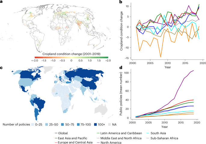
Figure 1a presents high-resolution maps at 10 × 10 km² pixel levels to capture heterogeneity within countries and across time on the basis of the spatial and temporal richness of the pixel-level data. To construct this map, we took average values over three-year windows (2001–2003 and 2017–2019) to minimize potential variability and possible year-specific spikes that may not be representative, or missingness of data due to the cloud cover for a specific pixel in a given year or possible measurement errors. The figure reveals substantial spatial heterogeneity, with the largest positive changes most pronounced in North America (especially Canada), Eastern Europe, Central Asia and parts of South and East Asia, probably reflecting effective management practices, sustainable intensification or agri-environmental policies. Negative changes are more pronounced in sub-Saharan Africa and scattered regions of South America and the Middle East, probably reflecting ongoing land degradation, climatic stress or low institutional capacity. Some countries, such as India and the USA (Midwest), show mixed changes with some parts improving and others declining. These spatial dynamics highlight the importance of using high-resolution maps instead of relying solely on country-level averages, which can mask localized degradation or improvement.

The patterns we observed closely align with previous studies for several regions and countries (for example, Europe, North America, southern Africa and Sahel regions, Latin America, and Southeast Asia, including China) but deviate for others (for example, India)^{48,58,59,60,61,62}. These differences may arise because most prior studies assess only ‘greening’ trends using direct measures of normalized difference vegetation index or EVI, without explicitly accounting for climatic and management effects. In such cases, observed greening or browning may be driven by agricultural intensification or climate change^62,63. Our measure accounts for these influences, capturing intrinsic land productivity. Overall, these global patterns highlight both progress and persistent challenges in cropland sustainability and provide a descriptive foundation for our policy impact analysis.

In Fig. 1b, we illustrate spatiotemporal variation in cropland condition relative to an early-period baseline across global regions. The global trend shows gradual improvement with modest overall recovery in cropland condition worldwide. However, at the regional level, trajectories reveal several heterogeneities. For example, North America, East Asia and Pacific, Europe and Latin America exhibit steady improvement in cropland condition over time, with some fluctuations but a broadly positive trajectory. In contrast, sub-Saharan Africa, the Middle East and South Asia mostly show persistently deteriorating conditions with considerable fluctuations, highlighting the dynamic nature of cropland condition in areas facing environmental and socio-economic pressures. Overall, this regional breakdown highlights areas with persistent vulnerabilities and consistent improvement beyond static global averages.

Finally, we explored the relationship between cropland condition measures and two key agricultural performance indicators: TFP and yield. We found strong positive associations between cropland condition and both yield and TFP across countries (Supplementary Figs. 4 and 5). In particular, countries with better cropland condition tended to exhibit higher average yields and TFP growth, suggesting that our measure captures meaningful variation in agricultural performance. However, this relationship is not uniform for all countries, especially for yield. For example, in countries such as Ethiopia, we observed a substantial increase in yields over time, while cropland condition has remained flat or declined (Supplementary Figs. 4 and 5). These divergences may suggest that yield improvements in some contexts may be driven by input intensification or short-term factors⁶⁴, rather than sustainable improvements in land quality. Overall, these patterns support the validity of cropland condition as a proxy for land-based productivity improvements, net of climatic variability and external input intensification.

Quantifying public policies

With regard to public policies, we focused on the government-led agri-environmental policies implemented within the administrative boundaries of countries¹⁰. These policies are of different types, ranging from legislative command-and-control measures to payment-based policies and various combinations of frameworks and monitoring policies (see Supplementary Table 2 for example policies). Moreover, while some of these policies directly aim to improve cropland condition (for example, soil erosion control or fertilizer regulation for soil health), others are more indirectly relevant (for example, biodiversity or forest conservation) (Supplementary Table 2). For the policy heterogeneity analysis, we categorized them into four groups: (1) soil and land-use regulations, (2) input-related policies (for example, fertilizers and agro-chemicals), (3) forest and biodiversity policies and (4) agri-environmental payment schemes (Fig. 8). While the policy database may not be exhaustive, it aims to comprehensively cover the most relevant policies over the period considered (Supplementary Fig. 6). We considered about 4,700 public agri-environmental policies implemented all around the world during the period 2001–2019.

Measuring these policies is not trivial due to the absence of a widely accepted policy indicators. The major limiting factors are multi-dimensionality in policies (multitude of instruments, exemptions, phase-in periods and accompanying measures), identification issues (the ability to attribute observed changes to actual policies instead of other factors) and data coverage and availability (including the tedious process of collating policy documents), inter alia^65,66. To overcome this, existing research usually relies on some outcome-based data, such as pollutant emission data^67,68, or the sheer number of policies to construct a proxy measure^32,69.

Here we began with a simple cumulative count of the policies that countries have implemented over the past two decades (2000–2019). While counting the number of policies may not be a perfect measure of policy, it can be a surprisingly good indicator of countries’ ‘policy effort’. For example, it is rare for a country to implement just one very large and ambitious policy; rather, countries often design and implement a bundle of many different policies, targeting different actors and regions (for example, see ref. ³³ for Brazil’s forest policies). In addition, countries may make many changes to their policies to achieve their goals (for example, see ref. ³² for climate policies). In our analysis, we have shown that the number of public policies is also strongly correlated with other policy-relevant indicators, such as budget, implementation abilities and human development required for policy design and implementation, implying that the number of policies matters (Supplementary Fig. 1).

However, this approach has clear limitations, as not all policies are equal in terms of coverage, budget or implementation process. To further improve our measurement of policies, we used two alternative policy measures. First, we constructed several policy indices by using the World Bank’s WGIs and the International Monetary Fund’s EPE^34,35. The WGIs are proxies for countries’ implementation capacity and institutional characteristics, while the EPE implies their policy budgets. We first normalized each WGI and EPE indicator to a scale of 0 to 1 and used them as weights for the policy variable. We then created a composite index by taking the average of all weighted policy variables (that is, the sum of policy number interacted with each indicator), as our main specification. Second, we used a policy measure that assigns each country to the treatment group if it has at least one public policy and treats it as a control otherwise. We also directly counted policies within each category (above) to capture variation in policy intensity across policy types.

Econometric approaches

The identification of the causal effect of national agri-environmental policies comes with a formidable empirical challenge due to non-random policy implementation and various natural and anthropogenic confounding factors^37,69. Here we describe the regression models used to deal with the identification issues faced in this study. To account for the potential confounding factors, we employed two state-of-the-art econometric methods: the border-region-based difference in discontinuities^36,37 and the entire-country-average-based spatial difference in differences^38,39. For the difference in discontinuities, we combined two cutting-edge econometric methods—regression discontinuity design and spatial difference-in-differences—leveraging on their respective fundamental advantages. First, in the context of regression discontinuity design, we relied on the assumption that two sides of countries’ borders are naturally comparable within the closely proximate border area—providing a typical ‘natural experiment’ setting^37,70,71. We then linked this to the difference-in-differences approach, which assumes that countries’ public policies are implemented over a specific time period, allowing us to detect changes in cropland condition after policy implementation³⁷. Combining the strengths of both methods, we employed a so-called difference-in-discontinuities design to estimate the causal effect of policies right around the international country borders³⁷. The key benefit of this design is that many international borders are naturally divided into two similar parts, where close to the border, both border sides are probably environmentally comparable, making them plausible counterfactuals for each other. We estimated the following regression equation:

Y_ibt denotes the cropland condition outcome (obtained from equation (1)) at pixel i in year t along the border of b country pair. This is constructed from the 83 million 1 × 1 km² grid-cell–year cropland condition measurements during 2001–2019. A higher Y_ibt implies improved cropland condition and vice versa. The term α_s(i,b)t indicates the border segment along the border by year fixed effects. The border segment is constructed by dividing the country borders into bins of narrower border segments on a half-degree grid (55 km). This allows direct cross-border comparisons not only at the borders that have patches of cropland on either side of the border but also at those with patches not necessarily close to each other. Each pixel is then assigned to the closest border point, which belongs to one of the border segments. D_it is the country treatment of interest, with countries with more cumulative policies taking the value 1 and countries with less cumulative policies taking the value 0 at the given border b. This variable is constructed for both weighted and non-weighted policy measures. β denotes the coefficient of interest, interpreted as the average treatment effect of the policy measure. X_i stands for the time-invariant spatial variables: distance to border (from each side), longitude, latitude and a cross-term. Finally, Z_ct represents country-level characteristics such as GDP, share of agriculture in GDP, population density, population growth, HDI, corruption, rule of law, political stability, accountability and environmental expenditures, and ε_it is an error term. These time-varying variables control for pixel- or country-level confounding factors. δ and γ are vectors of coefficients on X_i and Z_c. A full description and sources of all variables can be found in Supplementary Table 3. As our analysis relied on difference in discontinuities, we were able to account for many time-invariant confounders³⁷. By further controlling for time-varying country characteristics, we accounted for country-specific common shocks—for example, sudden changes in a country’s GDP.

Our analyses using border discontinuities in policies and cropland conditions relied on a number of important assumptions that motivated different placebo and sensitivity checks. Among the multiple robustness checks, we first estimated ‘placebo’ discontinuities by artificially shifting all borders by 5, 10 and 15 km both inwards and outwards from their original location. Our findings indicate no or less discontinuity at these placebo borders, reflecting the fact that only actual political borders are relevant (Extended Data Fig. 2). As a further robustness check, border discontinuities were estimated separately by increasing the optimal border bandwidth by 10 km (to 36 km) or decreasing it by 10 km (to 16 km). Our findings are again consistent with changes in optimal bandwidth (Extended Data Fig. 3). In addition, we performed several parallel trend tests and showed that future policies do not predict past cropland condition using policy leads. This test implies that our results are unlikely to be driven by reverse causality—that is, changes in cropland condition that led to new policies (Extended Data Fig. 4a,b).

The cropland discontinuities at international borders allowed us to focus on changes that occurred in generally similar agricultural conditions (unlike the country-level analysis). For example, near most international borders, soil types, rainfall and temperature are quite similar on each border side. However, this does not hold true everywhere, as borders sometimes follow mountain ranges, rivers and other geographic features that constitute natural discontinuities⁷². As a robustness check, we estimated a set of specifications using only observations from borders without natural discontinuities (Extended Data Fig. 5). We also performed a covariate balance test to check whether time-varying observables vary across international borders. The test result indicates insignificant differences between the control and treatment groups (Supplementary Table 5).

While this method potentially identifies the causal effect of policies, locations near the international border may not be representative of the cropland condition of the overall country. To address this limitation, we expanded beyond border areas, extracted aggregated country-level average cropland conditions and linked them with countries’ public policies. To construct a feasible counterfactual, we first sorted countries relative to their neighbours in terms of the number of policies implemented and then designated them as treated if they had more cumulative policies than their neighbours in each particular year. This enabled us to establish a plausible counterfactual among neighbouring countries with relatively similar environmental conditions. We then applied generalized difference in differences to detect the change in cropland condition attributable to implemented policies by estimating the change in cropland condition from the pre-policy to the post-policy implementation period. Here, the following equation was estimated:

Here Y_ct represents country-level average value of the cropland condition outcome for country c in year t (obtained using equation (1)). The sample size was determined by aggregating the annual maximum EVI from the entire country for each year from 2001 to 2019 and averaging at the country level (n = 3,040). D_ct is the country treatment of interest, where countries take value 1 if they have more cumulative policies than the average cumulative policies of all their neighbours and otherwise take value 0 for the given year t. Z_c controls for the country characteristics listed above for equation (2). Finally, α_c is the group (country) fixed effects controlling for all approximately fixed confounding factors that differ between countries, whereas τ_t is the year fixed effects, which controls for all period-specific common shocks. We estimated this model with the standard two-way fixed effects model³⁸. As discussed above, our results are also not specific to border regions, but country-level difference-in-differences estimates that do not rely on borders show the same patterns that we estimated in higher-resolution areas close to countries’ borders. To further test the robustness of the obtained effects, we performed various robustness checks and placebo tests to corroborate our findings. For example, we estimated the effect of policy leads on past cropland condition outcomes to understand whether future changes in policies affect past changes in cropland condition. We found no significant coefficients, implying that the parallel trend assumption holds (Extended Data Fig. 4b). We also further controlled for dominant crop types (Supplementary Fig. 7).

To approach country-level analysis from a different empirical perspective, we also estimated the dynamic difference-in-differences method^39,42. Here we applied two measures of policies. First, we used a general binary measure where countries are automatically assigned to the treatment group if they have implemented at least one cropland-condition-relevant public policy and remain in the control group until they have implemented at least one policy. Second, we classified policies into four types (Fig. 8) and counted policies within each category to capture variation in policy intensity across policy types. While this alternative policy measure deviates from our two previous methods, it offers us three important advantages. First, it enables us to explicitly test for the presence of the effects of policies during the pre-policy implementation period. Second, it provides important evidence that our findings are not prone to an artefact of a specific policy measure. Third, defining the treatment group on the basis of no policy instead of fewer policies might provide a more precise treatment estimate, albeit very local. We specifically used the event-study estimator by De Chaisemartin and D’Haultfoeuille^39,73. We set up our regression model as follows:

Here σ_τ and ϑ_τ correspond to the coefficients of the leads and lags of the treatment, respectively. All other terms are as in equation (3), apart from the treatment assignment procedure. Here we measure treatment D_c in two ways. First, beginning with the year 2001, each country is assigned to the treatment group if it has implemented at least one cropland-relevant public policy and remains in the control group until it has implemented at least one. In this case, the coefficient of D_c shows the average overall effect of policies in year-specific event-study estimates. Second, we categorized policies into four groups as discussed in section 2.2 and counted policies within each category. Here, in the spirit of a heterogeneity-robust difference-in-differences framework, treatment intensity is measured as the number of policies within each policy category, allowing us to estimate the marginal effect of an additional policy. Both country and year fixed effects are included, and standard errors are clustered at the country level. The added advantage of this method is its robustness to heterogeneous treatment effects across groups and over time periods, while still relying on the parallel trend assumption. Moreover, besides being an alternative policy measure, it allows us to explicitly test for the presence of the policy effects in the period prior to policy implementation (Fig. 8 and Extended Data Fig. 6). It further works well with unbalanced panels, wherein the outcome may be affected by the lagged treatment.

As a further robustness check, we also increased the policy threshold to at least three or more policies. This allowed us to check the sensitivity of our results to the chosen threshold levels (Supplementary Fig. 8). Another important insight we gained here is that there is a continuous yearly effect of policies on cropland condition. This provides insights into how the effect of public policies on cropland condition accumulates over time, rather than occurring immediately after policy implementation. For example, the positive changes in cropland condition caused by policies may mature slowly and take some time before being fully observable. To understand this better, we attempted to detect changes in cropland condition in response to implemented policies using policy lags. Our results reveal that the estimated policy effect steadily increases over time, which aligns with our expectation that the estimated policy effect accumulates over time (Supplementary Fig. 9).

Reporting summary

Further information on research design is available in the Nature Portfolio Reporting Summary linked to this article.