Estimation of direct and indirect polygenic effects and gene–environment interactions using polygenic scores in case–parent trio studies

Ethics section

This work used datasets from the UKB⁵³, the SPARK consortium¹³, Research Match: Genes and Environment Autism Research Study (GEARS) study and the GENEVA study^14,15. The UKB (https://www.ukbiobank.ac.uk) is under application no. 17731 and was approved by the North West Multi-centre Research Ethics Committee under reference no. 21/NW/0157. All participants provided written informed consent to participate. The SPARK and the GEARS studies used extant genomic and newly collected prenatal environmental data, using the GEARS environmental questionnaire, from participants enrolled in the SPARK study. The SPARK-integrated whole-exome sequencing (iWES) v3 dataset was generated from the SPARK study, led by researchers at Boston Children’s Hospital (study reviewed and approved by the institutional review board (IRB) of WIRB Copernicus Group). The GEARS study was reviewed and approved by the Johns Hopkins Bloomberg School of Public Health (protocol nos. IRB00007694 and IRB00021723) IRB. Written informed consent was obtained from all participants included in the analysis. These data are owned and distributed by the Simons Foundation Autism Research Initiative (SFARI). Aligning with the Common Rule definition of human research, as of March 2025, SFARI does not require IRB approval for requests of de-identified dataset biospecimens, including the SPARK iWES v3 and GEARS datasets. The GENEVA study was reviewed and approved by the IRB of each participating site, including the Johns Hopkins Bloomberg School of Public Health (protocol no. RPN 91-06-10-03-2).

Modeling direct genetic effects and gene–environment interactions

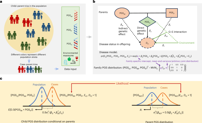
We assumed that PGSs for the index condition and other traits of interest can be evaluated for family trio participants, using published meta-data from prior association studies. Our goal is to investigate the association of these PGSs with an index condition, such as ASD, using case–parent trios. In a trio, let PGS_C, PGS_M and PGS_F denote the PGS values of the child, mother and father respectively. In addition, let D_C denote the binary outcome status of the child. We assumed that i = 1, …, N families have been sampled following the case–parent trio design. We also assumed that a set of environmental exposures, denoted by E_iC, has been ascertained for each child across the different families. We assumed that prospective disease risk of the child in the population follows a log-linear model:

Here pr is probability, \({\beta }_{{\rm{G}}}\) is the direct genetic effect (DE), β_GE is the vector of PGS × E interaction effects, β_E is the vector of main environment effects and T refers to a vector transpose. In equation (1), we assumed no indirect genetic effects, that is, within each family the parental PGS values affect only the child’s disease risk mediated through the child’s own PGS value, but we relaxed this assumption later (see subsequent sections and Supplementary Note 1). In addition, this model incorporates family-specific intercept terms, α_i, without any further assumption about their distribution, thereby allowing disease risks to vary arbitrarily across families. We used the log-linear model because it yielded closed-form estimators and allowed for the direct estimation of RR parameters, which are more interpretable in many epidemiological contexts. Although logistic regression is more commonly used—primarily because it constrains predicted probabilities between 0 and 1—it estimates ORs, which may be less intuitive. For rare diseases such as the developmental conditions studied here, the RR and OR tend to converge, making the two models nearly equivalent in practice. Although logistic regression is standard in case–control designs, prior studies^38,54 have shown that the log-linear- model is more suitable for case–parent and case-only designs, and rare disease assumptions are commonly invoked for comparing estimates with those from the logistic model.

We assumed that the joint distributions of PGS across families in the underlying population follow trivariate normal distributions of the form:

Here the correlation of 0.5 between PGS values of individual parents and children followed from Mendel’s law of inheritance. We allowed family-specific mean (μ_i) and variance (\({\sigma }_{i}^{2}\)) terms without imposing any assumptions about their distributions. We assumed that, within a family, PGS for the parents were independently distributed.

We have explained here how a model of equation (2) can flexibly account for both population structure and assortative mating. We conceptualized a sampling mechanism where, for each family sampled, we assumed that it belongs to a unique subpopulation of ‘homogeneous’ families with distinct genetic ancestry and trait characteristics influencing assortative mating. The number of these subpopulations can be arbitrarily large, making each subpopulation at an extremely fine level. It is assumed that random mating occurs within these homogeneous fine-level subpopulations, implying that the PGS correlation between partners is zero within these subpopulations, but not necessarily across them. We observed that the framework has similarity with classic models for assortative mating⁵⁵ which also assume random mating in a generation conditional on trait characteristics. Finally, we assumed \({{\bf {E}}_{i{\rm{C}}}} \perp ({{\rm{PG}}{\rm{S}}}_{i{\rm{C}}},{{\rm{PG}}{\rm{S}}}_{i{\rm{M}}},{{\rm{PG}}{\rm{S}}}_{i{\rm{F}}})\), but allow the distribution E_iC to remain unspecified. From a population perspective, this assumption can again be viewed as gene–environment independence within highly homogeneous subpopulations, but the model can still accommodate gene–environment correlation at the population level which may arise due to population substructure and assortative mating.

Retrospective likelihood and parameter estimation

The retrospective likelihood for the case–parent trio data in each family i can be decomposed into an offspring’s (L_iC) and a parent’s (L_iP) component as:

Under the above model, the likelihood components associated with children \({(L}_{i{\rm{C}}})\) and parental PGS \(({L}_{i{\rm{P}}})\) data for each family can be derived in terms of the following normal distributions (see Supplementary Note Section 1 for detailed derivation):

and

Maximum-likelihood estimation based on \(L=\displaystyle {\prod }_{i=1}^{N}{L}_{i}\) can be complex due to the presence of large dimensional nuisance parameters \({({\mu }_{i},{\sigma }_{i})}_{i=1}^{N}\). Instead, we proposed a combination of likelihood-based and moment-based estimation. First, we observed that the likelihood \({L}_{{\rm{C}}}=\displaystyle {\prod }_{i=1}^{N}{L}_{i{\rm{C}}}\) is informative for estimating \({\beta }_{{\rm{G}}}\) and \(\bf{\upbeta }_{\rm{GE}}\), but one complication is that it requires estimates of family-specific variance parameters \({\sigma }_{i}^{2}\). We then observed that, under the above model, the PGS values for two parents within each family are expected to have identical distribution and, thus, \({\hat{\sigma }}_{i}^{2}=0.5{({{\rm{PG}}{\rm{S}}}_{i{\rm{M}}}-{{\rm{PG}}{\rm{S}}}_{i{\rm{F}}})}^{2}\) provides an unbiased estimator for \({\sigma }_{i}^{2}\), i = 1, ‥. N. We can then obtain estimates of \({\beta }_{{\rm{G}}}\) and \(\bf{\upbeta }_{\rm{GE}}\) based on the likelihood L_C with plugged-in values for \({\hat{\sigma }}_{i}^{2}\). Under the above framework, we have shown that the final estimator can be derived in an analytical form as a solution to a weighted least-square problem as:

where \({\upbeta}={({\upbeta}_{\rm{G}},{{\mathbf{\upbeta}}_{\rm{GE}}^{\rm{T}}})}^{{\rm{T}}}\), \({\bf{E}}=({\bf{E}}_{1}^{\rm{T}},\cdots ,{\bf{E}}_{n}^{\rm{T}})^{\rm{T}}\), \({\bf{E}}_{i}=(1,{\bf{E}}_{i{\rm{C}}}^{{\rm{T}}})^{{\rm{T}}}\), \(\hat{\bf{W}}={\rm{diag}}({\hat{\sigma }}_{1}^{2},\cdots ,{\hat{\sigma }}_{n}^{2})\), \({\mathbf{Z}}=2({{\rm{PG}}{\rm{S}}}_{1{\rm{C}}}-{\mu }_{1{\rm{C}}},\cdots ,{{{\rm{PG}}{\rm{S}}}_{{\rm{NC}}}-\mu }_{{\rm{NC}}})^{{\rm{T}}}\) and \({\mu }_{i{\rm{C}}}=0.5({{\rm{PG}}{\rm{S}}}_{i{\rm{M}}}+{{\rm{PG}}{\rm{S}}}_{i{\rm{F}}})\).

In the special case when no gene–environment interaction terms are incorporated, the estimate of the DE of a PGS takes the simple form:

It is noteworthy that the numerator of equation (4) forms the basis of the pTDT test¹². In pTDT, the numerator is normalized by the variance of average PGS values of the parents across families. However, our derivation of equation (4) suggests that obtaining an unbiased estimate of effect size for the PGS in TDT-type analysis requires normalization of the transmission disequilibrium statistics, that is, the numerator, by an estimate of within-family variance. Intuitively, in all ascertained designs, such as case–control and case–parent trio studies, association tests effectively compare PGS values between cases and suitable controls or pseudo-controls. The observed mean difference in PGS reflects both the true effect size (\(\beta\)) and the variance of the PGS in the sampled population. As PGS variance differs between unrelated and related individuals—especially in the presence of population structure—even a fixed effect size can yield contrasts of different magnitudes across designs. Therefore, to obtain a consistent and interpretable estimate of \(\beta\), it is necessary to standardize the contrast using an appropriate variance term specific to the design.

We also note that the general form of equation (3), which incorporates gene–environment interactions, has an intuitive interpretation. The term \({\bf{E}}^{{\rm{T}}}{\bf{Z}}\) essentially represents the sample covariance between the transmission disequilibrium statistic and the environmental covariates across families. Under the null of no gene–environment interaction, transmission within a family is expected to be independent of family-level or parent-specific environmental factors (for example, maternal diet). Our derivation shows that departures from this null expectation in case–parent trio data provide evidence of gene–environment interaction on the multiplicative scale. However, we note that such transmission-based tests may not be appropriate when the environmental factor reflects a child’s own trait value, because these values can remain correlated with the child’s PGS even after conditioning on parental PGSs.

Incorporating indirect parental genetic effects

Next, we extend equation (1) to incorporate indirect parental genetic effects as:

where \({\beta }_{{\rm{M}}},{\beta }_{{\rm{F}}}\) capture indirect effects of parental PGS on the disease risk of the children not mediated through the children’s genotypes.

The likelihood components associated with children (L_iC) remain unchanged after incorporating the indirect genetic effects. We show, however, that the conditional distribution of PGS values in the mother or father in the ith ascertained family, when parental effects are incorporated, needs to be updated as \({L}_{i{\rm{P}}}=[{\mathrm{PGS}}_{i{\rm{M}}/i{\rm{F}}}|{{E}_{i{\rm{C}}},D}_{i{\rm{C}}}=1]\)\(\sim N\left({\mu}_{i}+{\sigma}_{i}^{2}\left[{\beta}_{{\rm{M}}/{\rm{F}}}+0.5({\beta}_{\rm{G}}+{\mathbf{\upbeta}}_{\mathrm{GE}}^{\bf{T}}{\bf{E}}_{{i}{\rm{C}}})\right],{\sigma}_{i}^{2}\right)\). Now we observed that, unlike the previous setting, here the two parents within a family could have asymmetrical distribution depending on the difference in the magnitude of their IDEs (\({\beta }_{{\rm{M}}}\) and \({\beta }_{{\rm{F}}}\)). We can exploit this parental asymmetry in PGS distribution to derive an estimator for the difference of parental indirect genetic effects (δ-IDE) as:

We further showed, in the presence of indirect effects, an approximately unbiased estimator for \({\sigma }_{\mathrm{sum}}^{2}/N=\displaystyle {\sum }_{i=1}^{N}{\sigma }_{i}^{2}/N\) can be derived as:

Furthermore, when the indirect effects of parental PGSs is incorporated, we observed that the form of the estimates of direct effect parameters β as shown in equation (3) remains unchanged, but the estimates \({\hat{\sigma }}_{i}^{2}\), i = 1, .‥ N in defining the weight matrix \(\hat{\bf{W}}={\rm{diag}}({\hat{\sigma }}_{1}^{2},\cdots ,{\hat{\sigma }}_{N}^{2})\) needs to be modified as \({\hat{\sigma }}_{i}^{2}=0.5[(\mathrm{PGS}_{i{\mathrm{M}}}-{\mathrm{PGS}}_{i{\mathrm{F}}})-\displaystyle {\sum }_{i=1}^{N}({\mathrm{PGS}}_{i{\mathrm{M}}}-{\mathrm{PGS}}_{i{\mathrm{F}}})/N]^{2}\) to obtain more accurate estimator of the quantity \({{\bf {E}}^{\rm{T}}}{\bf{WE}}\).

Equation (6) provides an intuitive test for asymmetrical indirect parental effects. In ancestrally homogeneous populations, allele frequencies are generally expected to be equal across sexes, so the expected difference in PGS between mothers and fathers is 0. Assortative mating induces within-pair covariance but does not alter this expectation. Thus, any nonzero mean difference in case–parent trios can signal asymmetrical IDE of parental PGS on offspring risk. However, if population-level mean PGS values differ by sex in the parental population, for example, due to asymmetrical selection, then we expect \(E({\rm{PG}}{{\rm{S}}}_{i{\rm{M}}}-{\rm{PG}}{{\rm{S}}}_{i{\rm{F}}}|{D}_{i{\rm{C}}}=1)={(\mu }_{{\rm{M}}}-{\mu }_{{\rm{F}}})+{\sigma }_{i}^{2}{\delta }_{{\rm{MF}}}\), where \({\mu }_{{\rm{M}}}\) and \({\mu }_{{\rm{F}}}\) denote the PGS mean for males and females in the underlying population. Thus, if sex-specific allele frequency for certain traits is suspected for the parental generation, we may further use an external dataset to obtain the difference in PGS between women and men to center our estimate of the indirect effect as:

In our autism application, we used data from the UKB to obtain external estimates of male–female differences in PGS values for various secondary traits and used them to carry out sensitivity analyses for the detected δ-IDEs.

Detailed derivations of all mathematical results and asymptotic variance estimators are presented in Supplementary Note 1.

Simulation studies

We conducted three types of simulation studies to evaluate the performance of the proposed method under complex population substructure and assortative mating. In the first setting, we simulated PGS values in >1 million randomly sampled trios from trivariate normal distribution based on equation (2) and disease status in children under the full model equation (5), and then further selected families with affected children (D = 1). We varied \({\rho }_{{\rm{G}}}={\rm{cor}}({\alpha }_{i},{\mu }_{i})\) to create different scenarios of population-stratification bias, with a value of 0 indicating no relationship between variation in disease risk and PGS distribution across the underlying substructure—a scenario where we do not expect any bias in population-based association studies. For the investigation of gene–environment interactions, we incorporated a binary (\({E}_{1}\)) and a continuous (\({E}_{2}\)) variable in the disease model. We allowed complex interrelationships among baseline disease risk \(({\alpha }_{i})\), PGS mean (\({\mu }_{i}\)) and exposure means (\({\gamma }_{i1}\) and \({\gamma }_{i2}\)) across families, in manners known to affect the estimation of gene–environment interactions using unrelated individuals⁵⁶.

We designed the second simulation setting to investigate the robustness of different methods for estimation of simulated effects of EA–PGS, a score that is known to be highly confounded with environmental factors due to population substructure^57,58 in the UKB study (www.ukbiobank.ac.uk). We built EA–PGSs using 4,483 independent SNPs (r² < 0.05 within 250 kb) and weights reported in previous work (PGS Catalog ID: PGS002440)⁵⁹ for the UKB participants. To simulate geographical population structure, we matched unrelated UKB males and females within assessment centers (UKB field ID 54) and by birth locations defined by north and east coordinates (UKB field IDs 129 and 130). In addition, we matched pairs based on both geographical proximity and similarity in EA (UKB field ID 6138) to simulate the additional effect of assortative mating. For each matched pair of UKB participants, we simulated children by generating their individual genotype values based on Mendel’s law of transmission. We further simulated children’s disease status based on equation (5), where a ‘hidden’ environmental variable, defined as the average of BMI values (UKB field ID 21001) of the two parents, was introduced to influence disease risk.

In the third setting, we used an existing tool snipar¹⁷ to simulate genotype data for 100,000 families across 1,000 independent SNPs, incorporating 20 generations of assortative mating with the parental phenotype correlation at 0.5, and a continuous phenotype influenced by direct genetic effects and assortative mating. To simulate children’s disease status, we used equation (5), including children’s PGS and parental indirect genetic effects, as well as mid-parental phenotype residuals regressing out parental PGS values as a family-level covariate to create an assortative mating effect in children’s disease outcome.

We also conducted additional simulation studies to evaluate potential effects of selection bias on parameter estimates associated with DEs and IDEs obtained from PGS-TRI (Supplementary Figs. 1–3). Details on all simulation settings, including the matching algorithm used for the UKB simulation, can be found in Supplementary Note 2.

Data analysis for application of PGS-TRI to ASD

We next demonstrated the application of PGS-TRI by analyzing genotype and epidemiological data available on n_trio = 18,383 case–parent trios from the SPARK study¹³ (https://sparkforautism.org/) (Supplementary Table 1). The key objectives included: (1) obtaining transmission-based estimates of the DE of the most advanced ASD–PGS to date built from prior studies, and comparing such an effect size from that reported from prior case–control studies; (2) assessing the portability of European-derived PGSs to non-European populations across ancestry groups and continuum of genetic ancestry; (3) evaluating the association of PGSs for multiple neurocognitive traits with ASD risk using the proposed transmission-based method; (4) characterizing the nature of interaction of ASD–PGS and prenatal exposure on ASD risk; and (5) discovering potential new associations of ASD risk with DEs and δ-IDEs of PGSs for gene-expression and obesity-related metabolite traits. We allowed the ancestry group of each family to be determined by the ancestry group of their offspring (Supplementary Table 1). Families where parents and the offspring share the same genetic ancestry group are defined as homogeneous families (N_homo = 15,876). For most of the analyses presented here, we used homogeneous families; however, for evaluating portability of PGS across the genetic ancestry continuum, we included all 18,383 trios.

Specifically, we examined ASD risk associated with DEs and IDEs of pre-constructed PGSs for ASD¹⁸ and 11 other cognitive and mental health-related traits that have been previously studied for potential links to ASDs^{12,16,60,61,62}, including EA⁶³, schizophrenia⁶⁴, strictly defined lifetime major depressive disorder⁶⁵, bipolar disorder⁶⁶, bipolar disorder I⁶⁶, bipolar disorder II⁶⁶, neuroticism⁶³, insomnia⁶³, chronotype⁶³, BMI⁶³ and ADHD⁶⁷ across different ancestry groups. The PGS for ASD itself were defined based on the largest GWAS to date conducted by the iPSYCH consortium and involved a total of 26,637 SNPs. We standardized all the PGSs across the continuum of genetic ancestry by mean adjustment⁶⁸ of the raw PGSs against the top five genetic PCs, using the 1000 Genomes Project and Human Genome Diversity Project (1kGP + HGDP)⁶⁹ as a reference dataset and then divided the PGSs residuals by ancestry-specific standard errors obtained from the reference dataset. This allowed interpretation of underlying risk parameters, that is, RRs, in a standard unit scale across ancestries.

We further examined ASD–PGS by context interactions, defined by the genetic distance on the continuous scale among all populations. Here genetic distance⁴⁶ is the Euclidean distance of the top 5 genetic PCs between each ASD child and the center of 98 unrelated Finnish individuals from 1kGP + HGDP to represent the PGS training population (north European) from the iPSYCH consortium. Using the homogeneous families, we further examined gene–environment interactions with several prenatal environmental factors, information being collected in SPARK participants using questionnaires designed by the GEARS study. Finally, we examined the association of ASD risk with genetically predicted levels of gene expression and metabolites using thousands of genetic scores generated by the OMICSPRED project²⁹. Here the underlying hypothesis is that genetically predicted biomarker levels, as captured by the underlying PGSs, could affect ASD risk through DEs or IDEs. We did note a caveat that, because the PGSs for biomarkers have been derived based on adult samples, the DEs of PGSs on children’s outcome are possible only if the same PGSs also predict biomarker levels in the fetal state and/or early childhood. Anticipating limited power for this analysis, we included only those biomolecular traits predicted with accuracy, R² ≥ 0.1, by the underlying genetic scores according to the internal validation in OMICSPRED and those included at least 5 SNPs in the underlying model. This criterion resulted in the evaluation of a total of 4,907 gene-expression levels and 27 highly correlated obesity-related metabolites. Additional details of data preprocessing and covariate coding can be found in Supplementary Note 3.

Data analysis for application of PGS-TRI to OFCs

We also applied PGS-TRI to investigate the polygenic risk of nonsyndromic OFCs using case–parent trio data from the GENEVA study^14,15. This analysis included a total of 778 European and 1,126 east Asian ancestry trios (see Supplementary Tables 11 and 12 for the distribution of trios by subtypes and exposure). We used these trio data to examine the effects of a predefined OFC–PGS on the risk of OFCs across different subtypes and ancestry groups, and its interaction with prenatal exposure to maternal smoking, maternal alcohol consumption, use of multivitamins during pregnancy and prenatal environmental tobacco smoke exposure^47,70. PGS for cleft lip with or without cleft palate (CL/P) were constructed using 24 SNPs and their respective weights sourced from the PGS Catalog^27,28. We standardized the OFC–PGS by ancestry-specific standard errors obtained from the 1000 Genomes Phase 3 Project⁶⁹. Finally, we also examined the risk of OFCs (CL/P) associated with the DEs and δ-IDEs of genetically predicted gene expressions and metabolite levels using genetic scores generated from the OMICSPRED project²⁹. Additional details of data preprocessing and covariate coding can be found in Supplementary Note 3.

Statistics and reproducibility

Our proposed method, PGS-TRI, was applied to estimate direct and asymmetrical indirect genetic effects and to assess gene–environment interactions (including ASD–PGS by context interactions) for all PGSs and genetically predicted transcriptome-wide and metabolome-wide traits within the SPARK consortium and GENEVA study. All hypothesis tests were two sided and based on Wald’s test statistics. Data analysis code to reproduce the results is available in our GitHub repository at https://github.com/ziqiaow/PGS.TRI and https://github.com/ziqiaow/PGS-TRI-Analysis and via Zenodo at https://doi.org/10.5281/zenodo.19189683 (ref. ⁷¹) and https://doi.org/10.5281/zenodo.19353771 (ref. ⁷²).

Reporting summary

Further information on research design is available in the Nature Portfolio Reporting Summary linked to this article.