Allocation and characterisation factors for absolute environmental sustainability assessment

Allocation factors

We determine the allocation factors for economic sectors across geographical scopes (e.g. countries or regions), based on theories of distributive justice. Theories of distributive justice postulate that a just allocation is always human-centric⁴. Although economic sectors are not human entities, they create value for humans. Hence, we determine allocation factors with the two-step approach proposed by Hjalsted et al.⁴: First, we allocate a share to the geographical scope, based on the share of global population living within the geographical scope. This allocates an equal share to each individual human, following the distributive justice theory of Egalitarianism⁴. Second, we allocate a share of the geographical scope’s allocated share to each economic sector within the geographical scope, based on the value that the economic sector generates for humans living in the geographical scope relative to the value generated by all sectors within the geographical scope, following the distributive justice theory of Utilitarianism⁴.

An economic sector generates direct and indirect value from both consumption and production perspectives. From the consumption perspective, direct value is generated when an economic sector’s output is directly consumed by the final consumer – such as individuals, households, and governmental institutions, who gain utility from the output. Indirect value is generated when the sector’s output is used by the sector’s downstream supply chain to produce output, which in turn is consumed by the final consumer. The sector’s downstream supply chain comprises other economic sectors in the same or other geographical scopes. The sum of direct and indirect consumption-based value is the total consumption-based value generated by an economic sector. We approximate the direct and total consumption-based value generated by an economic sector using the economic indicator of final consumption expenditure (FCE), defined as the monetary expenditure on goods and services for final use by individuals, households, governments, and non-profit institutions.

From the production perspective, direct value is generated within the sector, for example, by paying wages to its employees. Indirect value is generated as the sector’s input is produced by the sector’s upstream supply chain, which generates value within itself, for example, by paying wages to their employees. The sector’s upstream supply chain comprises other economic sectors in the same or other geographical scopes. The sum of direct and indirect production-based value is the total production-based value generated by an economic sector. We approximate the direct and total production-based value generated by an economic sector using the economic indicator of gross value added (GVA), which represents the monetary value of goods and services produced by the sector minus the monetary value of intermediate inputs used in production.

Mathematical formulation of allocation principles

We define four allocation principles to determine the allocation factor for a sector-scope pair \(({j}^{* },{s}^{* })\), where \(j\)* is an economic sectors from the set of sectors \({\mathscr{J}}\) and \(s\)* is a geographical scope from the set of geographical scopes \({\mathscr{S}}\). The set of sectors \({\mathscr{J}}\) and geographical scopes \({\mathscr{S}}\) are determined by an input-output model of the global economy that serves as the data source to which the allocation principles are applied.

We define the allocation principles following the two-step approach by Hjalsted et al.⁴. Accordingly, we obtain the allocation factors \({SoSO}{S}_{j* ,s* }^{p,q}\) for the sector-scope pair \(({j}^{* },{s}^{* })\) and for the four allocation principles differing between consumption and production value perspectives, \(p\in \left\{{\rm{cons}},\,{\rm{prod}}\right\}\), and direct and total value perspectives, \(q\in \left\{{\rm{direct}},{\rm{total}}\right\}\):

In Eq. 1, \({SoSO}{S}_{r}\) is the share of global population living in a geographical scope \(r\) (cf. Eq. 2) and \({{SoSOS}}_{j* ,s* ,r}^{p,{q}}\) is the share of value generated within \(r\) by the sector-scope pair \(({j}^{* },{s}^{* })\) (cf. Eqs. 3 and 4).

In Eq. 2, \({PO}{P}_{r}\) denotes the population of geographical scope \(r\) and \({PO}{P}^{{\rm{global}}}\) the global population.

The value-share \({{SoSOS}}_{j* ,s* ,r}^{p,{q}}\) is determined for the four allocation principles. Consequently, the value-share \({{SoSOS}}_{j* ,s* ,r}^{p,{q}}\,\) corresponds to the share of final consumption expenditure or gross value added in \(r\), for consumption or production-based perspectives, respectively, that is directly, or directly and indirectly (total) generated by \(({j}^{* },{s}^{* })\) (cf. Eqs. 3, 4).

In Eq. 3, \({{FCE}}_{j* ,s* ,r}^{q}\) is the final consumption expenditure generated by \(({j}^{* },{s}^{* })\) in \(r\) considering direct and total value generated \(q\in \left\{{\rm{direct}},{\rm{total}}\right\}\), and \({{FCE}}_{r}\) is the sum of direct final consumption expenditure in \(r\) across all sector-scope pairs \((j,s)\), where \(j\in {\mathscr{J}}\) and \(s\in {\mathscr{S}}\). In Eq. 4, \({{GVA}}_{j* ,s* ,r}^{q}\) is the gross value added generated by \(({j}^{* },{s}^{* })\) in \(r\) considering direct and total value generated \(q\in \left\{{\rm{direct}},{\rm{total}}\right\}\), and \({{GVA}}_{r}\) is the sum of direct gross value added in \(r\) across all sector-scope pairs \((j,s)\). Direct final consumption expenditure and direct gross value added can be directly obtained from the input-output model.

The total final consumption expenditure and total gross value added are obtained by scaling the direct final consumption expenditure and direct gross value added, respectively (cf. Eqs. 5, 6).

In Eq. 5, the scaling factor \({s}_{j* ,s* ,r}^{{\rm{FCE}}}\) captures the consumption-based value generation of the downstream supply chain that is induced by the sector-scope pair’s \(({j}^{* },{s}^{* })\) output. The scaling factor is calculated following the method of Oosterhoff et al.⁶, which is omitted here for brevity. In Eq. 6, the scaling factor \({s}_{j* ,s* ,r}^{{\rm{GVA}}}\) captures the production-based value generation of the upstream supply chain that is induced by the sector-scope pair’s \(({j}^{* },{s}^{* })\) input.

In Eq. 7, \({m}_{j* ,s* }\left({{GVA}}_{j* ,s* }^{{\rm{direct}}}\right)\) is the type I gross-value-added multiplier for each \(({j}^{* },{s}^{* })\), as proposed by Keček et al.²⁰. The type I gross-value-added multiplier captures the production-based value generation of the upstream supply chain that is induced by the sector-scope pair’s \(({j}^{* },{s}^{* })\,\) input, without disaggregating by the geographical scope \(r\). In Eq. 7, \({\alpha }_{r,j* ,s* }\) is the share of inputs into \(({j}^{* },{s}^{* })\,\) from geographical scope \(r\).

In Eq. 8, \({\varphi }_{i,r,j* ,s* }\) is the share of inputs into \(({j}^{* },{s}^{* })\,\) from each sector-scope pair \((i,r)\).

In Eq. 9, \({z}_{i,r,j* ,s* }\) is an input from the sector \(i{\mathscr{\in }}{\mathscr{J}}\) in geographical scope \(r\,\epsilon \,{\mathscr{S}}\), \({{GVA}}_{j* ,s* }^{{\rm{direct}}}\) is the direct gross value added of \(({j}^{* },{s}^{* })\), and \({T}_{j* ,s* }\) is the total input into the sector-scope pair \(({j}^{* },{s}^{* })\), which is calculated with Eq. 10.

Since the total consumption-based and production-based values of a sector include the downstream and upstream supply chains, respectively, the same economic value can be attributed to multiple economic sectors. Consequently, allocation factors are not additive across sectors, and their sum generally exceeds one. As a result, aggregating allocation factors—such as when accounting for the same sector across multiple geographic scopes—can lead to double counting of consumption-based or production-based values.

This limitation can be illustrated using a simplified economy consisting of only one geographical scope and of two economic sectors A and B, where sector A supplies sector B. The total consumption-based value of sector A consists of its own direct consumption-based value plus the share of sector B’s consumption-based value that is attributable to inputs from sector A. In contrast, the total consumption-based value of sector B equals only its direct consumption-based value because it does not supply any downstream sector.

If the total consumption-based values of sectors A and B are summed, the resulting value exceeds the economy’s overall consumption-based value, which is simply the sum of the sectors’ direct consumption-based values. The excess arises because part of sector B’s value is counted twice: once as part of sector B’s own total value and again as part of sector A’s total value. An analogous overlap occurs for production-based values, where upstream supply chain relationships lead to double counting.

Consequently, the sum of value-shares \({{SoSOS}}_{j* ,s* ,r}^{p,{q}}\) exceeds 1, when total value generation is considered, as the same value is attributed to multiple economic sectors. For the same reason, the sum of allocation factor \({SoSO}{S}_{j* ,s* }^{p,q}\) resulting from the value-share also exceeds 1.

Application of allocation principles

We obtain all data required for calculating consumption-based and production-based values from the multi-regional input-output database, EXIOBASE 3.9.6²¹, which is an input-output model of the global economy, and by using the most recent industry-by-industry database for 2022²¹. Therefore, we determine the allocation factors for 163 economic sectors across 44 countries and 5 Rest-of-World regions, i.e., 49 geographical scopes, as included in EXIOBASE 3²². For population data, we use country-specific figures provided by the World Bank for 2022²³ for all countries that are explicitly defined in EXIOBASE 3²². We align the Rest-of-World regions in EXIOBASE 3 with corresponding World Bank regional classifications²⁴ (cf. Table 1). For each Rest-of-World region, we include the population data of all countries that are not explicitly defined in EXIOBASE 3²².

Characterisation factors

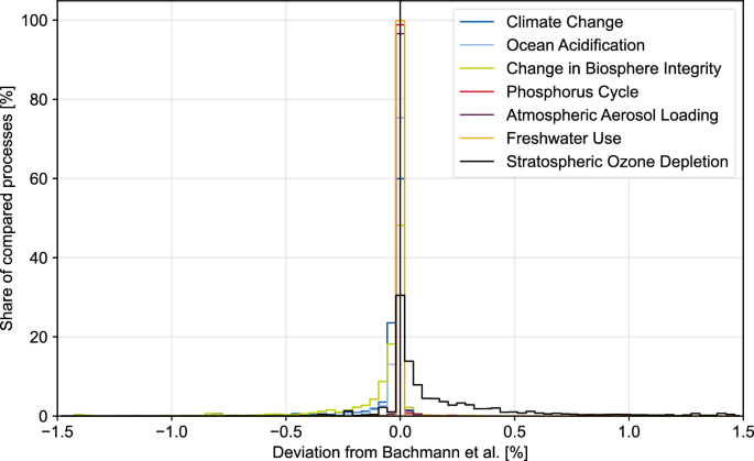
Our calculation of the characterisation factors primarily builds on the work of Ryberg et al.¹⁵ and Bachmann et al.⁸ Ryberg et al. developed characterisation methods to obtain characterisation factors for planetary-boundary-based life cycle impact assessment, while Bachmann et al.⁸ adapted these characterisation methods and published characterisation factors for all 2080 elementary flows included in ecoinvent v3.5¹³. In this work, we further adapt the characterisation method for land-system change and apply the resulting characterisation methods to all 2684 elementary flows within standard and prospective ecoinvent v3.10.1.

In ecoinvent, elementary flows are distinguished by the type of mass or energy emitted or extracted, the main compartment of emission (i.e. air, water or soil) or extraction (i.e. natural resources), and additional sub-compartments. The standard ecoinvent v3.10.1 database¹³ and the prospective ecoinvent v3.10.1 databases, generated using premise 2.1.9¹⁹, include 2648 and 2684 elementary flows, respectively. The increase in elementary flows between v3.5 and v3.10.1 is due to additional masses, energies, compartments and sub-compartments.

Furthermore, v3.10.1 includes changes to the name, compartment and sub-compartment of elementary flows compared to v3.5. When changes between v3.5 and v3.10.1 involve only synonyms, new or renamed compartments, or sub-compartments, we transfer the original characterisation factors from v3.5 to the corresponding updated elementary flows in v3.10.1. To address flows newly added or previously unaccounted for in v3.5, we introduce characterisation factors for the following planetary boundary categories: climate change, biosphere integrity, ocean acidification, stratospheric ozone depletion, and atmospheric aerosol loading. We introduce new characterisation factors for land-system change by characterising land occupation. To account for the burden on the nitrogen cycle, we introduce a new elementary flow and characterisation factor. For the planetary boundaries on climate change and biosphere integrity—each of which is defined by two control variables—the dataset includes characterisation factors for only one control variable per boundary. Additionally, regionalized burden categories included in the planetary boundary framework are not represented in the dataset.

Climate change, change in biosphere integrity and ocean acidification

For the planetary boundary categories, climate change, change in biosphere integrity and ocean acidification, we add characterisation factors for ‘Carbon dioxide, to soil or biomass stock’ to the compartment ‘soil’ by copying and negating the characterisation factors for ‘Carbon dioxide, fossil’ to ‘air’, in accordance with other life cycle impact assessment methods, such as the Environmental Footprint 3.1²⁵ Furthermore, we assign a characterisation factor for ‘Ketene’ to ‘air’ by copying the factor from ‘NMVOC, non-methane volatile organic compounds’ to ‘air’, as ‘Ketene’ does not have a specified carbon content.

Bachmann et al.⁸ calculate characterisation factors for the burden of land occupation on change in biosphere integrity using the method provided by Galán-Martín et al.²⁶, which uses data for mean species abundance loss from Hanafiah et al.²⁷. However, Hanafiah et al. do not provide data for all types of land occupation present in the v3.10.1 database. Hence, we map the types of land occupation introduced between v3.5 and v3.10.1 to the classifications used by Hanafiah et al., as detailed in Table 2. If multiple values are provided by Hanafiah et al. for a given type of land occupation, we use the maximum values as a conservative approximation.

Stratospheric ozone depletion

We characterise ‘Dichloromethane’ to ‘air’ using the characterisation method provided by Ryberg et al.¹⁵, assuming an atmospheric lifetime of dichloromethane of 0.5 years²⁸ and a fractional release ratio of 1.

Atmospheric aerosol loading

We characterise the elementary flow ‘Carbon’ to ‘air’ with the characterisation factor for ‘Carbon-14’ to ‘air’. Furthermore, we assign a characterisation factor to ‘Ketene’ to ‘air’ by copying the factor from ‘NMVOC, non-methane volatile organic compounds’ to ‘air’ and the sub-compartment ‘unspecified’, as ‘Ketene’ does not have a specified carbon content.

Nitrogen cycle

Nitrogen application to soil via fertilisers impacts the planetary boundary category for the nitrogen cycle¹. However, nitrogen application to soil via fertilisers is not included as an elementary flow in ecoinvent, but as a technosphere flow^13,29. To assess the burden on the nitrogen cycle, we introduce the new elementary flow ‘N-supply’, emitted to the compartment ‘soil’. This elementary flow is added to all processes that supply nitrogen application via fertilizers as a technosphere flow. Specifically, we consider all processes in ecoinvent v3.10.1¹³ that include the term “nutrient supply” in their process name and provide either ‘organic nitrogen fertiliser, as N’ or ‘inorganic nitrogen fertiliser, as N’ as the technosphere flow. Hence, if a process supplies 1 kg of nitrogen to an agricultural system, 1 kg of the ‘N-supply’ elementary flow is emitted to the compartment ‘soil’. We characterise the elementary flow ‘N-supply’ to the compartment ‘soil’ with the factor 1e-9 to convert from kilograms to teragrams.

Land-system change

We provide a novel set of characterisation factors for land-system change to enable the comparison of the environmental burden on land-system change with the SOS defined by Doka et al.¹⁶. We characterise all elementary flows representing anthropogenic land occupation in ecoinvent v3.10.1 with the factor 1e-12, converting from square meters to million square kilometres, except the elementary flows beginning with ‘Occupation, forest’, ‘Occupation, grassland, natural’, and ‘Occupation, seabed’, as well as the elementary flows ‘Occupation, unspecified, natural (non-use)’ and ‘Occupation, shrub land, sclerophyllous’. We exclude these elementary flows since the SOS defined by Doka et al.¹⁶ corresponds to the land that is available for anthropogenic occupation. Land that is available for anthropogenic occupation is calculated as the total area of ice-free land surface minus the minimum area that should be covered by forest¹⁶. The minimum area that should be covered by forest is retrieved from Steffen et al.¹. Hence, we do not characterise ‘Occupation, forest’, conservatively assuming that it reflects existing forest cover rather than anthropogenic forest cover expansion. We do not characterise ‘Occupation, grassland, natural’, ‘Occupation, unspecified, natural (non-use)’ and ‘Occupation, shrub land, sclerophyllous’, assuming that no forest cover has been removed from these natural land-systems by anthropogenic activity. We further do not characterise ‘Occupation, seabed’ because it does not involve the occupation of terrestrial land area.