
Appendix: External dataset for additional validation
Data description
To further strengthen the reliability of the reported performance metrics and to explicitly address concerns related to possible overfitting or data leakage, additional experiments were conducted using an independent public dataset, namely the Smart Manufacturing IoT–Cloud Monitoring Dataset, available on Kaggle (https://www.kaggle.com/datasets/ziya07/smart-manufacturing-iot-cloud-monitoring-dataset). This dataset was designed to support research in industrial IoT analytics, particularly for real-time monitoring, predictive maintenance, and anomaly detection in smart manufacturing systems. It contains approximately 100,000 multivariate sensor records collected at one-minute intervals from 50 distinct machines, including measurements such as temperature, vibration, humidity, pressure, and energy consumption. In addition to continuous sensor streams, the dataset provides machine operational states (e.g., idle, running, failure), anomaly indicators, and a supervised target variable (maintenance_required) that specifies whether maintenance intervention is required. The combination of dense temporal sampling, heterogeneous sensor modalities, and operational annotations makes this dataset a realistic and challenging benchmark for validating time-series learning models under noisy IoT conditions.
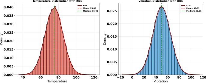
This dataset exhibits characteristics commonly observed in real industrial deployments, including sensor noise, operational regime shifts, and imbalanced maintenance events, all of which pose challenges for robust model generalization. By applying the same DGGO-LSTM pipeline, preprocessing strategy, and evaluation protocol used in the main experiments—without dataset-specific tuning—this external validation aims to assess the transferability of the proposed approach across different IoT domains. The use of an entirely independent manufacturing dataset provides additional evidence that the high predictive accuracy reported in the primary results is not attributable to favorable data partitioning or information leakage, but rather reflects the stable learning behavior and generalization capability of the proposed DGGO-based optimization framework when applied to diverse multivariate IoT scenarios. Figure 22 displays the probability density distributions of temperature and vibration measurements using histograms overlaid with Kernel Density Estimation (KDE) curves. These visualizations provide insights into the statistical characteristics of the respective datasets, revealing patterns of central tendency and variability. In both subplots, the KDE curves closely follow a bell-shaped form, suggesting near-normal distributions. The proximity of the mean and median lines in each plot further supports this symmetry, indicating minimal skewness in the data. Such analysis is instrumental in understanding the underlying behavior of thermal and mechanical parameters in system monitoring contexts.

Density plots of temperature (left) and vibration (right) with KDE overlays and central tendency markers.
Figure 23 presents a time series analysis of four key operational parameters—temperature, vibration, humidity, and pressure—utilizing rolling statistical estimates to detect anomalies. For each variable, the plots display the raw signal over time, overlaid with a smoothed rolling mean to highlight local trends and mitigate short-term fluctuations. The shaded envelope captures variability using rolling standard deviation bands. Anomalies, indicated as extreme values beyond statistical thresholds, are prominently visible in the temperature and vibration plots, with 176 and 175 extremes detected respectively. In contrast, humidity and pressure remain within normal variability bounds, with no significant anomalies observed. This form of temporal analysis is critical in predictive maintenance applications, where early detection of abnormal behavior can preempt costly system failures.

Rolling mean and anomaly detection across time series for temperature, vibration, humidity, and pressure.
Baseline model performance on the external dataset
To establish a transparent performance reference and to contextualize the effectiveness of the proposed DGGO-based optimization framework, several baseline deep learning models were evaluated on the Smart Manufacturing IoT–Cloud Monitoring Dataset using the same preprocessing pipeline, strict chronological data split, and evaluation protocol adopted in the main experiments. The considered baseline models include LSTM, Transformer-based Time Series Transformer (TST), RNN, CNN, and a feedforward ANN. Their predictive performance was assessed using multiple statistical indicators, including Mean Squared Error (MSE), Root Mean Squared Error (RMSE), Mean Absolute Error (MAE), Mean Bias Error (MBE), Pearson correlation coefficient (r), coefficient of determination (\(R^2\)), Relative RMSE (RRMSE), Nash–Sutcliffe Efficiency (NSE), and Willmott’s Index (WI), as summarized in Table 15.
As shown in Table 15, the LSTM model achieves the strongest overall performance among the baseline approaches, yielding the lowest MSE (0.0089), highest NSE (0.902), and the most favorable correlation metrics. Transformer-based and recurrent architectures also demonstrate competitive predictive accuracy, although with moderately higher error values. In contrast, CNN and ANN models exhibit comparatively weaker performance, particularly in terms of error-based and efficiency metrics, reflecting their limited capacity to model long-term temporal dependencies in multivariate IoT sensor streams.
Overall, these baseline results indicate that, while the external dataset poses realistic challenges such as sensor noise and operational variability, it does not trivially yield near-perfect predictions. This observation supports the validity of the dataset as a meaningful benchmark and establishes a robust reference against which the performance gains achieved by the proposed DGGO-optimized models can be fairly evaluated in subsequent analyses.
Figure 24 presents a heatmap of normalized performance metrics across five deep learning architectures: LSTM, Transformer (TST), RNN, CNN, and ANN. Each cell reflects the scaled value (ranging from 0 to 1) of a specific evaluation metric, enabling direct comparison of model behavior across multiple criteria. The normalization facilitates interpretation by standardizing disparate metric ranges, highlighting relative strengths and weaknesses. Error metrics (MSE, RMSE, MAE, MBE) show progressively lower normalized values from ANN to LSTM, while correlation-based metrics (r, \(R^2\)) and skill scores (NSE, WI) reveal inverse trends. Notably, LSTM achieves optimal scores in statistical and index-based measures but underperforms in error metrics, whereas ANN demonstrates the highest error rates but minimal predictive reliability. This visualization supports robust model selection by synthesizing multi-metric performance into a unified comparative framework.

Normalized comparison of model performance metrics across five deep learning architectures.
Comparative performance of binary feature selection optimizers
To further examine the robustness of the proposed feature selection strategy on the external Smart Manufacturing IoT–Cloud Monitoring Dataset, we compared the proposed binary Dynamic Greylag Goose Optimization (bDGGO) against several widely used binary metaheuristic optimizers, namely binary Harris Hawks Optimization (bHHO), binary Grey Wolf Optimizer (bGWO), binary Particle Swarm Optimization (bPSO), binary Bat Algorithm (bBA), binary Whale Optimization Algorithm (bWOA), and binary Biogeography-Based Optimization (bBBO). The comparison focuses on both predictive quality and selection parsimony, reporting the average error, average selected feature ratio (selection size), and fitness statistics (average, best, worst, and standard deviation). These metrics provide complementary evidence regarding (i) how accurately the selected feature subset supports prediction, (ii) how compact the resulting subset is, and (iii) how stable each optimizer is across repeated runs. The results are summarized in Table 16.
As shown in Table 16, bDGGO achieves the lowest average error (0.305) while simultaneously selecting the smallest average subset size (0.26), indicating a favorable balance between predictive accuracy and feature parsimony. Moreover, bDGGO produces the best fitness value (0.27) among all compared optimizers and maintains a relatively low fitness variability (standard deviation 0.195), suggesting stable convergence behavior. In contrast, several competing approaches (e.g., bPSO, bBA, and bWOA) tend to select substantially larger feature subsets while yielding higher average error and weaker fitness outcomes. Overall, these results support that the proposed bDGGO feature selection mechanism generalizes effectively to the external dataset and can identify compact informative feature subsets without compromising predictive performance.
Model performance after feature selection on the external dataset
To assess the impact of feature selection on predictive performance and to further evaluate the generalization ability of the proposed framework, the baseline learning models were re-trained and evaluated on the Smart Manufacturing IoT–Cloud Monitoring Dataset using the feature subsets selected by the proposed bDGGO algorithm. The same preprocessing pipeline, chronological data split, and evaluation protocol were preserved to ensure a fair comparison with the baseline results reported earlier. Performance was evaluated using multiple statistical indicators, including error-based metrics, correlation measures, and efficiency indices, as summarized in Table 17.
As shown in Table 17, all predictive models benefit noticeably from the bDGGO-based feature selection process, exhibiting consistent reductions in MSE, RMSE, and MAE compared to their corresponding baseline configurations. The LSTM model achieves the strongest overall performance, with an NSE of 0.927 and the lowest MSE (0.0058), indicating improved learning efficiency when redundant and less informative features are removed. Transformer and recurrent models also demonstrate meaningful gains, while CNN and ANN architectures show moderate but consistent improvement across all evaluation metrics. These results confirm that the proposed bDGGO feature selection mechanism effectively enhances predictive accuracy while preserving stable generalization behavior on an independent industrial IoT dataset, thereby reinforcing the credibility of the high-performance metrics reported in the main study.
Figure 25 provides a comparative overview of model performance metrics by displaying the mean values alongside their associated variability through error bars. The metrics—ranging from error-based measures (MSE, RMSE, MAE, MBE) to correlation coefficients (r, \(R^2\)), relative error (RRMSE), and efficiency indices (NSE, WI)—offer a multidimensional perspective on model accuracy and reliability. The line plot highlights the variation in predictive accuracy across different evaluation criteria, with RRMSE standing out due to its notably higher mean and wider spread, indicating its sensitivity to scale and error amplification. The inclusion of error bars enables visual assessment of metric stability and confidence, aiding in the interpretation of model robustness across diverse statistical dimensions.

Line plot of model evaluation metrics with mean values and error bars.
Figure 26 illustrates the distribution of nine evaluation metrics across different models using horizontally oriented box plots augmented with swarm plots. This layout enables a clear comparative analysis of central tendency, variability, and individual metric values. Each subplot corresponds to a specific metric—MSE, RMSE, MAE, MBE, Pearson’s r, \(R^2\), RRMSE, NSE, and Willmott’s WI—revealing how these metrics fluctuate among models. The compact horizontal orientation enhances readability of small differences in scale, particularly for low-variance metrics such as r and \(R^2\). The inclusion of swarm plots enriches the visualization by exposing the density and distribution of model-specific results around the median. This figure supports robust benchmarking by exposing both consistency and outliers in model evaluation across all key statistical dimensions.

Horizontal box and swarm plots for distribution of evaluation metrics across models.
Comparison of optimized LSTM models on the external dataset
To further investigate the effectiveness of the proposed Dynamic Greylag Goose Optimization (DGGO) algorithm in optimizing deep learning models, we compared the performance of LSTM models optimized using different metaheuristic algorithms on the Smart Manufacturing IoT–Cloud Monitoring Dataset. Specifically, DGGO+LSTM was evaluated against LSTM models optimized using Grey Wolf Optimizer (GWO), standard Greylag Goose Optimization (GGO), and Whale Optimization Algorithm (WOA). All optimized models employed the same feature subsets produced by their respective binary optimizers, identical preprocessing procedures, and the same chronological data split to ensure a fair and unbiased comparison. Performance was assessed using a comprehensive set of error, correlation, and efficiency metrics, as summarized in Table 18.
As reported in Table 18, the DGGO+LSTM model consistently outperforms all competing optimized configurations across every evaluation metric. In particular, DGGO+LSTM achieves the lowest MSE (1.55×10\(^{-5}\)) and RMSE (0.00395), alongside the highest correlation (\(r=0.971\)), coefficient of determination (\(R^2=0.968\)), and efficiency indices (NSE = 0.971, WI = 0.976). Compared to GWO-, GGO-, and WOA-optimized LSTM models, DGGO-based optimization yields both lower prediction error and improved stability, as evidenced by reduced bias and relative error measures. These results indicate that the proposed DGGO mechanism provides a more effective balance between exploration and exploitation during the optimization process, leading to superior convergence toward high-quality solutions.
Importantly, although DGGO+LSTM achieves very high predictive accuracy on this external dataset, the observed performance hierarchy across optimizers remains consistent and non-trivial, with clear performance gaps between methods. This consistency, together with the independent nature of the dataset and the controlled experimental protocol, supports the conclusion that the achieved performance gains reflect genuine optimization improvements rather than overfitting or information leakage.
Figure 27 depicts a dendrogram generated from hierarchical clustering applied to hybrid models combining LSTM with various metaheuristic optimization algorithms: DGGO, GWO, GGO, and WOA. The vertical axis represents the distance metric used to quantify dissimilarity between model outputs, enabling a data-driven grouping based on performance similarity. The close linkage between WOA+LSTM and GGO+LSTM indicates a high degree of similarity, followed by a moderate resemblance to GWO+LSTM. In contrast, DGGO+LSTM forms a distinct cluster, suggesting divergence in performance behavior. This hierarchical structure offers a visual taxonomy of model relationships, supporting comparative diagnostics and ensemble strategy formulation based on underlying metric proximities.

Hierarchical clustering dendrogram of hybrid LSTM models with different optimizers.
Figure 28 presents Q-Q (quantile–quantile) plots for nine commonly used model evaluation metrics: MSE, RMSE, MAE, MBE, r, \(R^2\), RRMSE, NSE, and WI. These plots assess whether the distribution of each metric conforms to a normal distribution by comparing the ordered sample values against theoretical quantiles. The linearity observed in most of the plots suggests that the residuals or metric values are approximately normally distributed, which is an important assumption for the validity of many statistical inference techniques. Minor deviations from the reference line in some metrics, such as MBE and RRMSE, may indicate skewness or outlier presence. This analysis facilitates the assessment of underlying assumptions required for parametric tests and model interpretability.

Q-Q plots for model evaluation metrics assessing normality of their distributions.
Statistical significance analysis on the external dataset
To further validate the robustness and generalizability of the proposed DGGO–LSTM framework, statistical significance testing was also conducted using the results obtained from the external dataset reported in the Appendix. As with the primary dataset, two complementary statistical analyses were employed: a one-way Analysis of Variance (ANOVA) to assess overall performance differences among methods, followed by pairwise nonparametric testing using the Wilcoxon signed-rank test.
ANOVA test results
A one-way ANOVA test was applied to the mean squared error (MSE) values obtained across the optimized models evaluated on the external dataset. The ANOVA results are reported in Table 19.
As shown in Table 19, the ANOVA test yields a statistically significant result (P<0.0001), indicating that there are meaningful performance differences among the evaluated optimization strategies on the external dataset. This confirms that the choice of optimization method significantly influences predictive accuracy beyond random variation.
Wilcoxon signed-rank test results
To further examine pairwise differences and specifically assess the performance gains achieved by the proposed DGGO–LSTM framework, Wilcoxon signed-rank tests were performed. This nonparametric test was selected due to its robustness to non-normal error distributions and its suitability for paired comparisons based on cross-validation results. The Wilcoxon signed-rank test results are reported in Table 20.
Figure 29 provides a comprehensive visual evaluation of the predictive performance and interrelations among the applied models. The two scatter plots in the top row display the model-wise distribution of the Root Mean Square Error (RMSE) and Nash–Sutcliffe Efficiency (NSE), respectively, highlighting variance and central tendency through the spread of blue data points. The bottom-left subplot illustrates a regression plot comparing observed versus predicted values across all models, with a reference line \(y = x\) in red, which serves to assess the predictive bias and alignment of estimations. Finally, the bottom-right subplot contains a heatmap summarizing the performance metric values for each model, with the intensity of green indicating superior performance and red denoting relatively lower accuracy. This integrative figure enables comparative analysis through both statistical distribution and model ranking, supporting a multidimensional performance appraisal.

Composite visualization of model performance via scatter plots, regression analysis, and heatmap summary.
Figure 30 presents a histogram-based comparative visualization of model outputs, structured to highlight the individual and overlapping distributions for each learning model. The figure incorporates histograms representing the data distributions associated with four distinct models—LSTM, RNN, CNN, and ANN—each denoted by different colors (blue, red, green, and magenta, respectively). These histograms not only visualize the frequency distribution of the data values for each model but also allow for a quick assessment of spread, central tendency, and outliers. The alignment of these histograms facilitates side-by-side comparison of the distribution characteristics across models, which is essential for identifying consistency or variability in prediction behavior among the learning algorithms.

Histogram comparison of output distributions across different models.
The Wilcoxon signed-rank test results demonstrate that DGGO–LSTM achieves statistically significant improvements over GWO–LSTM, GGO–LSTM, and WOA–LSTM on the external dataset, with all two-tailed p-values equal to 0.002 and well below the 0.05 significance threshold. The reported discrepancy values further indicate that the magnitude of the performance differences consistently favors DGGO–LSTM, reinforcing the statistical robustness and cross-dataset generalizability of the proposed optimization framework.