Coastal ecosystem degradation driven by decades of unregulated terrestrial mining

Study site

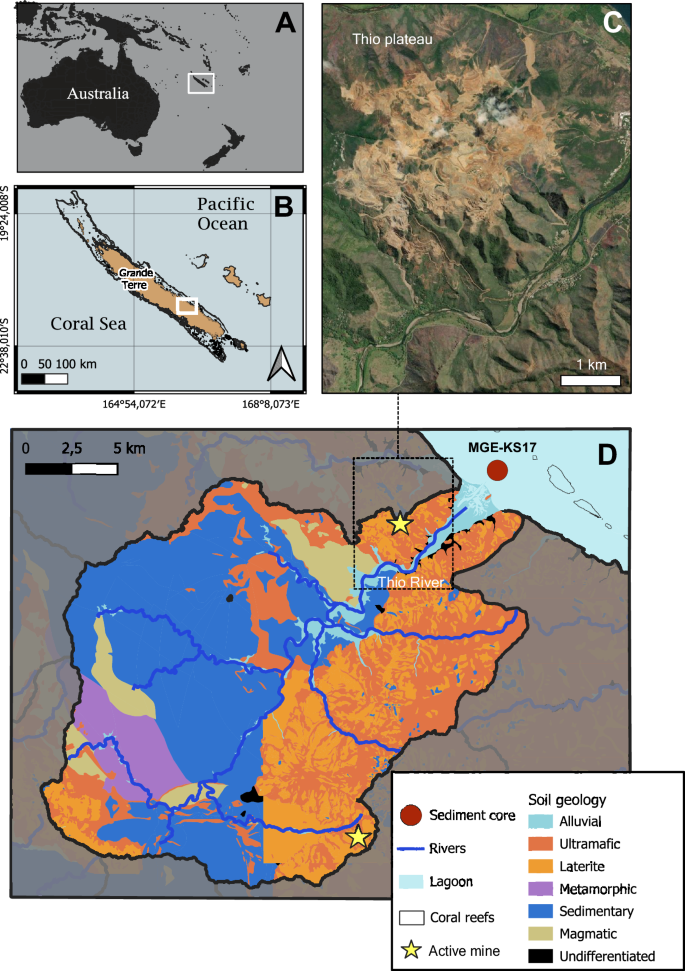
New Caledonia is a large microcontinental island located in the southwest Pacific Ocean (Fig. 6A). The climate is considered subtropical. It is separated into two main seasons: a dry season (May–October) and a wet season (December–March). During the wet season, especially in February–March, extreme events like tropical depressions and cyclones can lead to massive rainfalls and strong winds.

The alternative text for this image may have been generated using AI.

Maps of A New Caledonia in the southwest Pacific Ocean and B the Grande Terre Island. C Aerial view of the oldest mining site of Thio plateau, still active at the time of the sampling (Esri, Maxar, World Imagery basemap). D Simplified geological map of the Thio watershed (QGIS v.3.36.2 with shape files from https://georep-dtsi-sgt.opendata.arcgis.com/).

The Thio River is located on the southeast coast of New Caledonia (Fig. 6B). The watershed encompasses an area of 397 km² (Fig. 6D) and a population of approximately 2500 inhabitants. The low urbanisation and negligible agriculture in this area allow for disentangling the impacts of mining activities from other anthropogenic pressures. The mining activity (Fig. 6C) lies on ultramafic regoliths of several tens of metres that are classically composed of a saprolite unit overlaid by a laterite unit and are characterised by high concentrations of nickel, chrome and cobalt¹⁹. The right bank of the watershed is predominantly composed of an ultramafic geological setting, whereas the left bank is mainly composed of a volcano-sedimentary basement (at the origin of sedimentary and magmatic soil) (Fig. 6D). Those geological settings cover about 90% of the watershed surface area²³. The mouth of the river is connected to the second-largest lagoon in the world, which has been partly referenced on the UNESCO World Heritage list since 2008 for its exceptional marine biodiversity.

Historical background of the local nickel mining

The exploitation of mineral resources in New Caledonia began in 1864 with the discovery of a nickel- and magnesium-rich silicate rock, later named garnierite by the mining engineer Jules Garnier⁶⁰. Mining activities at Thio officially started in 1875, which makes this site the first nickel extraction site in the world. At that time, mining operations used shovels and pickaxes to extract green garnierite ores with nickel concentrations up to 12% from underground tunnels. The Société Le Nickel was created in 1880, marking a substantial milestone in the local mining industry. Around 1920, mining operations transitioned from underground methods to open-pit mining, which required the removal of vegetation and non-viable topsoil⁶¹. As a reflection of early globalisation, sailing ships were constantly waiting to export minerals to Europe and Japan.

The mechanisation of mining operations only began in 1950, introducing more efficient extraction techniques that enhanced topsoil removal and access to higher-grade saprolite⁶². Between 1950 and 1975, an estimated 1.125 million tons of waste rock were discharged annually into the Thio watershed, totalling 27 million tons over 25 years⁶³. This period also witnessed a considerable increase in nickel production, particularly during the ‘nickel boom’ from 1967 to 1971.

A critical turning point in the mining history of the Thio regions occurred in 1975 with Cyclone Alison, which caused a massive runoff of lateritic mining waste stored on mountain slopes since the 1950s. The cyclone caused severe flooding with red, muddy water, inflicting extensive damage to crops and homes and leaving a lasting mark on the local community’s collective memory⁶⁴. In response, Société Le Nickel, supported by ORSTOM (Office of Overseas Scientific and Technical Research, now IRD, Research Institute for Development) scientists, implemented a series of erosion control measures, including constructing waste rock dumps, replacing bulldozers with hydraulic excavators and trucks, improving water management systems with natural berms, gutters and settling basins, and re-vegetating previously mined areas. After 1985, further efforts were made to reduce the sediment discharge into the lagoon in compliance with broader environmental regulations, including the 1975 European directive and the national law on waste management and material recovery (n°75–633 of July 15, 1975). Since 2009, New Caledonia’s Congress has implemented a mining development plan and code that established environmental protection measures to promote the sustainability of mining practices. These regulations require environmental impact assessments, public consultations and the rehabilitation of degraded areas.

Sampling

The MGE-KS17 sediment core was sampled during the MARGEST (sedimentology, stratigraphy and neotectonics of the eastern margin of New Caledonia)⁶⁵ campaign at 1 km from the Thio River mouth (21°35,832′ S; 166°14,055′ E, Fig. 6D), 15 m water depth on April 22, 2022, using a Kullenberg piston corer equipped with a PCV (PolyVinyl chloride) tube, aboard the Research Vessel Alis. The core measured 226 cm and was divided on board into three sections, each less than one metre long, for immediate transport to a selected field laboratory. The core sections were subsampled into one-centimetre-wide layers by extruding the core from the PVC tube using calibrated sterilised plastic rings and sterilised inox cutting blades¹⁴. Each layer was subsampled for the following analyses. To optimise material usage, alternating layers were assigned to different analyses: one layer was used for foraminiferal examination, and the adjacent layer was used for sedaDNA analysis and environmental parameters. The inner part of the sediment layer was reserved for sedaDNA analyses to avoid contamination by the PVC core device and smearing due to core extrusion. Once the sediment layer was cut, the central part was immediately isolated and protected from external contamination using a sterile 6-cm Petri dish. About 15 g of sediment was sampled from each 1-cm layer using sterilised wooden tongue depressors. The samples were placed in plastic 50 mL deoxygenated cryotubes and immediately frozen in liquid nitrogen for transport before being stored at −80 °C for sedaDNA extraction. The remaining sediment of each slice was sampled for physicochemical analysis.

Sediment dating

The more recent sediments of the core (upper 150 cm) were dated using depth profiles of excess ²¹⁰Pb (²¹⁰Pbxs, a naturally occurring radionuclide) and ¹³⁷Cs (an artificial one)⁶⁶. Those two components were measured in approximately 5 g of dry sediment using a well-type, high-efficiency γ detector (Canberra, France)⁶⁷. Excess ²¹⁰Pb in sediments, ²¹⁰Pbxs, was calculated by subtracting the activity supported by its parent isotope, ²²⁶Ra, from the total measured ²¹⁰Pb activity. The sediment accumulation rate (SAR, expressed in cm yr⁻¹) was calculated from the decrease of ²¹⁰Pbxs with depth using the CFCS (constant flux and constant sediment model) and CIC (constant initial concentration model)⁶⁸. Six CIC ²¹⁰Pb ages have been selected to contribute to the final age model (Supplementary Table 1).

The oldest recovered sediments were dated using accelerator mass spectrometer standard radiocarbon methods on marine mollusc shells and a bulk assemblage of benthic foraminifera at AWI MICADAS⁶⁹. ¹⁴C ages were calibrated using CALIB 8.2 program⁷⁰ and MARINE20 calibration curve⁷¹ for radiocarbon ages older than 600 yrs BP (Supplementary Table 1). A regional marine reservoir correction of mean ΔR = 151 ± 32 yrs inferred from radiocarbon measurements in pre-bomb known-age shells and coral from the SW Pacific Ocean⁷² was applied. The two ¹⁴C ages above 130 cm produced higher values of ¹⁴C, suggesting post-bomb ages. Radiocarbon values and uncertainties were converted to calendar years using the CALIBomb program^73,74 by comparing our radiocarbon measurements to regional data collection from the Great Barrier Reef⁷⁵.

Finally, sediment ages were interpolated in order to build an accurate age model using the Bayesian age-depth modelling BACON software⁷⁶. The objective was to estimate the ages of sedimentary units, specifically unit II, where sediments produced a very diluted ²¹⁰Pb_xs activity and accumulated too few micro-shells to obtain enough material to measure a robust radiocarbon activity in the sample and a reliable fraction modern carbon (F¹⁴C) estimate because of strong terrigenous dilution. The modelling strategy was to propagate by BACON iterations the prior assumptions about accumulation rate from the base of the core (oldest layers) to the base of Unit II (93 cm) and then from the top core to the sediment layer above the Unit II (upper 40 cm) to determine ages just before and just after the sediment deposition of Unit II. The model also allowed to evaluate sediment accumulation rate, mean ages and uncertainties all along the core.

Physicochemical parameters

The sediment particle size (granulometry) was determined by analysing their scattering patterns using laser technology with a Mastersizer Hydro 2000S (Malvern Panalytical Ltd., Malvern, UK). The grain size was then categorised into clay (0–3.9 µm), silt (3.9–63 µm) and sand (63–2000 µm).

Elemental concentrations of Ag, Al, Cd, Co, Cr, Cu, Fe, Li, Mn, Ni, Pb, V, Zn, As, Mo, Sn, Sb, Ba and U were determined on freeze-dried sediment aliquots by inductively coupled plasma mass spectrometry (TQ-ICP-MS, iCAP TQ, Thermo Fisher Scientific, Waltham, CA, USA), following Siano et al.¹⁴. Each sample batch was processed alongside procedural blanks and certified international reference materials (CRM) MESS-4 and PACS-2 (National Research Council of Canada), undergoing the entire procedure, including digestion, elemental analysis and isotopic measurements. Mercury analyses were performed using a semi-automatic mercury analyser (AMA-254, LECO Corporation, St. Joseph, MI, USA) on freeze-dried sediment aliquots. Concentrations obtained for replicate measurements of the CRM MESS-4 corresponded to the recommended value (0.091 ± 0.009 μg g⁻¹).

Organophosphate ester (OPE) flame retardants and plasticisers are among the most widely distributed organic plastic additives in the environment⁷⁷ and were selected for analysis in this study. OPEs were analysed in 17 core horizons. Dry weight sediments (2 g) were sonicated with ethyl acetate/cyclohexane (80:20, v/v) after spiking with OPE labelled standards. Clean-up was performed using SPE-NH₂ columns with sequential elution in two fractions, and 18 different OPEs were quantified by isotope dilution liquid chromatography-tandem mass spectrometry (LC-MS/MS). The analytical procedure can be found more detailed in a previous work⁷⁷.

For organic matter content, samples were decarbonated by direct acidification with 1 mol L⁻¹ HCl in silver capsules and then dried in an oven for 16 h. The decarbonated samples were subsequently analysed using a Thermo Flash Smart Analyzer (Thermo Fisher Scientific), calibrated using aspartic acid, to measure both total nitrogen (TN) and particulate organic carbon (POC). Each sample measurement was corrected for the blank signal from the acidified silver capsule. Due to technical issues, 14 samples were lost.

Sediment source modelling

PMF (positive matrix factorisation) model, a receptor model-based source tracing method^78,79, was employed to quantify the relative contributions of ultramafic and volcano-sedimentary geological settings to sediment accumulation along the core. The PMF-5.0 model (U.S. EPA, https://www.epa.gov/air-research/positive-matrix-factorization-model-environmental-data-analyses) was applied on the concentrations of 20 major and trace elements and the grain size distributions across 62 sediment samples. The model decomposed these data into two matrices, representing sediment source profiles and relative contributions in each of the 62 samples analysed (Supplementary Table 3).

Foraminifera identification and SST reconstruction

To isolate benthic foraminifera, 126 samples containing the exact same amount of sediment (sampled with a normalised size tube, pressed upside down over the whole thickness and in the inner part of the selected one-centimetre-wide sediment layers), were preserved in 100 mL of ethanol. Once back in the lab, they were washed separately using demineralised water and sieved through mesh sizes of 300 and 150 μm, to only retain adult specimens. All the foraminifera present in the sediment samples were hand-picked under a binocular microscope using a fine paintbrush and placed on black numbered grids with double-sided adhesive tape for identification and geochemical analysis. It led to the picking of approximately 7000 foraminifera along the whole core, with an average of about 50–70 specimens per sample, although certain samples (10) presented a complete absence of foraminifera. Each foraminifera was identified at the genus level using a stereo zoom microscope (SMZ 171 with MLC-150C cold light, Motic, Kowloon Bay, Hong Kong), using the two main scientific local references published^80,81. The genus level was chosen to ensure consistent taxonomic identification across the numerous core samples, which varied in sediment quality and often contained partially damaged shells that limited reliable species-level determination. Due to its strong representation along the core, the benthic foraminiferal species Ammonia sp. was selected for Mg/Ca determination. Each point represents the average ratio concentrations analysed within the calcite of 5 specimens coming from the same sample (about 0.150 mg of calcite per sample). Prior to ICP-MS analysis, samples were weighed, washed in ethanol, rinsed with Milli-Q water and underwent an ultrasound bath for 5 min, before being dissolved in nitric acid (HNO3). The solutions obtained were analysed using the Perkin Elmer NexION 350× from the LAB’EAU in Ducos, New Caledonia. The system features a triple quadrupole configuration that enhances its ability to filter out interferences, providing accurate and reliable results⁸². To guarantee the precision and accuracy of the measurements, several quality control measures were implemented: internal standards (water), blank samples, certified reference materials (JCP-1 and JCT-1) and replicates. Precision was assessed by the relative standard deviation (RSD) of triplicate analyses and was maintained below 5% for all elements. Due to particularly elevated Mg/Ca concentrations measured in average on Ammonia specimens (around 70 mmol mol⁻¹) clearly largely adapted to a tropical environment, and despite very common Sr/Ca ratios analyzed on the same specimens (around 1000–1500 µmol mol⁻¹) the Mg-T equation established on the tropical species Baculogypsina sphaerulata was preferred to reconstruct Sea Surface temperature (SST) over time:

Using this last regression, the reconstructed temperature ranged from 16 to 27 °C (with a mean of 22 °C). The observed warming over the last two centuries is in good agreement with the observed temperature increase admitted for these regions of the Pacific since the beginning of the industrial revolution in 1850⁸³.

Extraction and amplification of sedimentary ancient DNA

SedaDNA was extracted from 73 samples obtained after core slicing. Samples were selected using a constant criterion (i.e. approximately every 2 cm up to a depth of 20 cm, and then every 4 cm, one sample over two, Supplementary Table 4) and collected along the core, in the centre of each slice (to prevent contamination). To follow specific precautions to avoid contamination with modern DNA of biological laboratories, extractions were done at the controlled atmosphere laboratory (LAC) of the University of Nouméa. This laboratory is an ISO 7 certified facility divided into four modules, including the ‘biology’ module, which is maintained under negative pressure, classified as P2, and equipped with two microbiological safety cabinets (PSM) compliant with EN 12469 standards. The agent conducting the extractions was dressed in a sterile and single-use suit, gloves, hairnet and mask (Supplementary Fig. 10). Each time, an extraction blank was performed to detect any potential contamination, resulting in 21 such negative controls. As recommended for sedaDNA studies⁸⁴, the DNAeasy Power soil kit (Qiagen N. V., Venlo, Netherlands) (lots n°17202244 and 17202245) was used on 10 g of wet sediment, following the manufacturer’s protocol. The kits were opened and handled in the LAC to ensure contamination-free processing. To avoid cross-contamination between samples, the extractions were carried out one by one, from the most ancient to the most recent sample, cleaning the entire material and working area between each using DNA away (Dominique Dutscher, Bernolsheim, France) and UV light.

For DNA amplification, the 18S rDNA V4 region was chosen to study the variation of microeukaryote diversity. At the relatively short paleo-timescale of a few centuries, this region has proven to better represent taxonomic groups than the shorter V7 region in a paleogenomic study¹⁴. DNA amplification was done using TAReuk454FWD1/TAReukREV3 primers⁸⁵ associated with GeT-PlaGe adaptors from GeT-Biopuces (INSA Toulouse, France). PCR mix included 6 µL buffer high fidelity 5×, 0.6 µL dNTP (10 mmol L⁻¹), 0.9 µL DMSO 3%, 1.1 µL forward primer (0 35 µmol L⁻¹), 1.1 µL reverse primer (0.35 µmol L⁻¹), 18 µL water, 0.3 µL Taq Phusion 2 U µL⁻¹ (Thermo Fisher Scientific) and 2 µL of sample, for a final volume of 30 µL. The amplification program consisted in an initial amplification at 95 °C for 30 s, 12 cycles of 98 °C for 10 s, 53 °C for 30 s and 72 °C for 30 s, then 18 cycles of 98 °C for 10 s, 48 °C for 30 s and 72 °C for 30 s, with a final extension of 72 °C for 10 min. Plates with caps were used to further limit external and cross-sample contaminations, and each well was opened one by one for reagent addition. Two amplification blanks were conducted to identify any potential contamination during the amplification process. Five amplifications were made per sample, checked by electrophoresis gels, and the DNA concentration was quantified using Qubit 4 (Thermo Fisher Scientific). As expected, a decrease in DNA concentrations was observed in deeper samples (Supplementary Fig. 11). The five PCR replicates were pooled before Illumina MiSeq sequencing using a standard V3 kit (2 × 250 bp) at the GeT-Biopuces platform.

Bioinformatic treatment

The pipeline SAMBA (v4, https://gitlab.ifremer.fr/bioinfo/workflows/samba) was used to process the raw sequences and construct a high-quality Amplicon Sequence Variant (ASV) dataset. Taxonomic assignment was performed using the PR² reference database (v5.0.0)⁸⁶. Total samples comprise 25,250 ASVs and 5,996,275 reads. As expected, variations of sequencing depth were observed across the samples, with a marked decrease at the end of the core corresponding to the older samples.

In order to compare samples despite the bias of variable sequencing depth (Supplementary Fig. 12), a rarefaction was performed at 40,000 reads. This threshold was arbitrarily chosen to keep every sample collected during the potential period of mining activities and to retain the samples in the first two portions of the core with the minimum read number (sample B02 at 70 cm depth, 40,610 reads). This method, done with rarefy_even_depth() function from phyloseq package⁸⁷, removed 17 low-read samples, resulting in the loss of 2,526 ASVs from the deeper section of the core (>164 cm). The rarefaction method was chosen for this study, despite the removal of samples, as it encompasses the entire mining history in terms of sediment ageing and is the strictest way to limit sequencing depth differences when using ancient DNA.

Across 23 negative controls (extraction and amplification blanks), 85 ASVs (213,299 reads in total, Supplementary Data 1) were detected, and all of these ASVs were conservatively treated as contaminants and removed from the dataset prior to downstream analyses. To focus on protists and fungi, ASVs assigned to non-eukaryotes (1056 ASVs), metazoans (518 ASVs), Streptophyta (176 ASVs), Ulvophyceae (67 ASVs), Florideophyceae (3 ASVs) and Sargassum (1 ASV) were excluded. After these taxonomic filters, the rarefied dataset was composed of 20,855 ASVs (83% of the initial dataset).

Functional assignments

The study of past communities using ancient DNA is highly influenced by the degradation of DNA over time. The amplicon sequencing method did not allow to build a pattern of DNA degradation with depth, as the amplification step removes modifications of the DNA, such as deamination, that are useful for estimating a degradation rate⁸⁸. Some microeukaryotes are capable of resting stages (e.g. cyst or spore)^11,89. This evolutionary capacity is advantageous in paleogenetic studies¹⁴, as the remaining cell protects the preservation of the DNA from external degradation factors. For this work, we focused on these taxa to provide a strict and consistent analysis of biological patterns. In order to highlight those taxa, an assignment based on the taxonomy of our ASVs was performed, using the traits ‘RestingStage’ from the functional database of Ramond et al.⁹⁰, supplemented with literature sources. Short 18S amplicons make species-level assignment unreliable, so we opted to assign ASVs at the genus level. For ecological analyses, we retained all genera for which at least one species is known to form resting stages. For instance, the genus Chaetoceros, which includes some species capable of forming resting spores, was considered a resting stage-forming genus regardless of the ASV-based species-level annotation. In the same way, the kingdom Fungi, known to form spores⁹¹, and the Apicomplexa classes Coccidiomorphea and Gregarinomorphea, known to form resting stages^92,93, were generally assigned as taxa capable of forming resting stages. We anticipate that this approach may lead to overestimating the number of ASVs capable of forming resting stages. Within the rarefied dataset, 19% of ASVs and 47% of the reads were annotated to taxa capable of forming a resting stage.

Biostatistical analyses

All statistical analyses were conducted in R v4.3.3⁹⁴. A clustering based on the concentrations of nickel and aluminium allowed the identification of five distinct groups of samples using the ctree() function from the partykit package v1.2-20⁹⁵. The identified groups were then correlated with sediment dating to associate each group with a specific time period. Three samples, however, were not clustered together with the others but instead appeared isolated between groups, which made it difficult to define a continuous chronological sequence (Supplementary Fig. 1). To maintain a clear and consistent temporal framework, these samples were not included in the definition of the groups. The resulting groups were referred to as ‘sedimentary units’.

Because our study relies on two distinct types of biodiversity data, we applied different but harmonised preprocessing strategies. For the ASV dataset, diversity metrics based on richness and presence–absence (e.g. alpha diversity and Jaccard dissimilarity) were computed on the non-rarefied count table but using approaches designed to account for methodological biases (e.g. corrected by sedimentation rates). This choice was made to retain the oldest samples, which yielded fewer than 40,000 reads and would otherwise have been excluded by rarefaction. The equivalent figure based on the rarefied dataset is available in the Supplementary Material to show that the results are qualitatively consistent (Supplementary Fig. 13). In contrast, all analyses relying on read abundances were performed on the rarefied dataset and expressed as relative abundances to ensure comparability among samples and minimise sequencing-depth bias. For the foraminifera dataset, the data are inherently low-dimensional and already limited in information content. Therefore, they were analysed as genus-level presence–absence data without further transformation.

The richness of the community was described using the number of ASVs and foraminiferal genera in each sample. Because richness measured in sedimentary archives can be artificially inflated by time-averaging effects when sedimentation rates are low, observed alpha diversity was corrected by sediment accumulation rate. The relationship between diversity and sedimentation rate was modelled using log-transformed values of both variables to account for their non-linear relationship and to reduce the influence of extreme values. As fossil diversity is expected to increase mechanically with the duration over which assemblages accumulate, independently of ecological processes, the residuals of this model were retained as a measure of sedimentation-corrected diversity. This approach removes the component of diversity explained solely by sediment accumulation and allows us to focus on temporal ecological changes not driven by variations in sedimentation rate⁹⁶. Several Podani indices were used to describe more precisely the variations of ASV richness along the core, including richness difference and ASV replacement^97,98. These indices, together with Jaccard dissimilarity, were computed using a moving-window approach rather than fixed temporal bins. For each sample, Podani indices and Jaccard dissimilarity were calculated by comparing that sample to the two immediately preceding samples in the core (e.g. the sample at 10 cm was compared to those at 12 and 14 cm). This approach ensures comparisons among samples that are close in depth and therefore more comparable in terms of DNA preservation and sedimentation rate, thereby limiting artificial richness differences driven by DNA degradation. Using a moving-window framework also smooths short-term variability and reduces sensitivity to uneven temporal resolution caused by variations in sedimentation rate and time averaging. As a result, the estimated richness difference, replacement and dissimilarity metrics are less affected by vertical mixing and uneven sample spacing than estimates based on discrete and irregular temporal bins. The relative abundance at the subdivision level was then used to assess variability in dominant groups of microeukaryotes along the core from the rarefied dataset.

Community variability along the core at the genus level was assessed through principal coordinates analysis (PCoA) with Jaccard dissimilarity using wcmdscale() function of vegan package v2.7-2. The influence of different factors (depth, unit, metallic composition, organic matter and source of sediment) was evaluated with a hierarchical partitioning, using rdacca.hp() function of rdacca.hp package v1.1⁹⁹. The contribution of each factor to the explained variance was quantified as the total contribution, including both its individual effect and shared effects with other factors. The temporal dynamics of microeukaryotic and foraminiferal genera along the core were analysed depending on their relative abundance and presence/absence, respectively. We acknowledge that robust species-level assignment could enhance our understanding of the specific effects of mining, providing additional ecological information, such as lifestyle, trophic strategy or physiological tolerance, which may differ among species within the same genus. Yet, the genus level was chosen for homogenisation with the foraminifera dataset and because amplicon sequencing with universal markers does not reliably support confident species-level assignments (e.g. ref. ¹⁰⁰). The randomness of the distribution was tested using the run.test() function from the tseries package for foraminiferal genera. To evaluate relative abundance differences between sedimentary units, Wilcoxon non-parametric tests (using the wilcox.test() function from the stats package) were conducted on each genus capable of resting stage and present in at least four samples (183 genera). Three tests compared sedimentary units III–IV, II–III and I–II, searching for significant changes in relative abundance across units. Resulting p-values were adjusted for multiple testing using the Bonferroni correction.

Long reads amplicon sequencing implementation for fungi identification

Because many fungal ASVs could not be assigned beyond the kingdom level, we performed long-read rRNA gene sequencing (SSU-V4 to LSU-D9^101,102) using PacBio Sequel. These long-read OTUs were then aligned to Illumina short-read ASVs using VSEARCH¹⁰³ to build sequence similarity networks, enabling taxonomic linkage between short- and long-read datasets (detailed method available in Supplementary Methods).