Phenomics-assisted Sparse Testing For Potato Breeding

Plant material and conventional phenotyping

In this study, we evaluated a potato population composed of 256 breeding clones and cultivars, fully listed in Supplementary Table S1. The plant material employed in the present study are in compilance with institutional, national, and international guidelines and legislation.

Field trials were carried out using incomplete block designs at two rural sites in southern Sweden: Helgegården (56$^{\circ }$00$^{\prime }$56$^{\prime \prime }$N/14$^{\circ }$03$^{\prime }$50$^{\prime \prime }$E) and Mosslunda (55$^{\circ }$58$^{\prime }$04$^{\prime \prime }$N/14$^{\circ }$06$^{\prime }$51$^{\prime \prime }$E). At Helgegården, trials took place in 2020 with 169 genotypes arranged in a 13 $\times$ 13 simple lattice design and evaluated in two replications. In 2021, trials at Helgegården included the full set of 256 genotypes, arranged in a 16 $\times$ 16 simple lattice design with two replications. At Mosslunda, a single trial was conducted in 2021 using the full set of genotypes and the same lattice design of Helgegården in 2021. Each location-year combination was treated as a unique environment for subsequent analysis.

The local growing season typically extends from late May through early September, lasting roughly 3.5 to 4 months. To capture environmental variation across sites and seasons, we obtained daily weather and elevation data using the EnvRtype R package v1.1.2¹⁸. Environmental covariates considered included: (i) temperature at 2 m ($^{\circ }$C); (ii) maximum temperature at 2 m ($^{\circ }$C); (iii) minimum temperature at 2 m ($^{\circ }$C); (iv) dew/frost point at 2 m (m/s); (v) downward thermal infrared (longwave) radiative flux; (vi) all-sky insolation on a horizontal surface; (vii) all-sky downward direct normal shortwave irradiance; (viii) all-sky photosynthetically active radiation (PAR); (ix) all-sky ultraviolet A irradiance (315–400 nm); (x) all-sky ultraviolet B irradiance (280–315 nm); (xi) precipitation (mm); (xii) evapotranspiration energy flux at the surface; (xiii) specific humidity at 2 m (kg water/kg total air); (xiv) relative humidity at 2 m; (xv) root-zone soil wetness (0–100 cm); (xvi) surface soil wetness (0–5 cm); (xvii) wind speed at 2 m (m/s); (xviii) precipitation minus evapotranspiration; (xix) vapor pressure deficit (kPa); (xx) photoperiod (h); (xxi) top-of-atmosphere radiation; (xxii) number of theoretical sunny hours per day under clear skies; (xxiii) temperature–humidity index 1¹⁹; (xxiv) temperature–humidity index 2²⁰; and (xxv) the ratio of PAR to temperature.

Despite the close proximity of the trial sites, they belong to different 0.5$^{\circ }$ grid cells in the NASA POWER database²¹, which may slightly differentiate the environmental data retrieved. To analyze seasonal patterns, monthly averages for each covariate were calculated for every environment. These values were visualized using heatmaps created with the pheatmap package v1.0.12²² in R v4.1.2²³. Pairwise Pearson correlations were also computed using the monthly means to examine similarities between environments. Additionally, daily temperature curves for 2020 and 2021 were plotted using ggplot2 v3.5.1²⁴ to depict temporal trends.

The set of conventional traits evaluated comprised total tuber weight (kg); tuber weight (kg) within defined size ranges (<40 mm, 40–50 mm, 50–60 mm, and >60 mm); and tuber starch content (%).

High-throughput phenotyping

For each field trial, we also evaluated image-based traits obtained from drone imagery collected at multiple time points in each environment (Table 1). All flights were conducted at an altitude of 30 meters. The UAV used was a DJI Mavic 2 Pro UAV, equipped with a 20 MP RGB camera.

Table 1 Time points for aerial image acquisition in each environment.

Drone image processing was carried out using the software Pysel (Phenoyard AB, Sweden), which included the following steps for each flight-environment combination: (i) orthomosaic generation; (ii) definition of experimental plots ; and (iii) extraction of plant measurements and vegetation indices, including: visible atmospherically resistant index (VARI), green-red ratio index (GRRI), canopy reflectance (CR), coverage, plant height, and leaf chlorophyll content.

For the vegetation indices VARI and GRRI, pixel-wise values were averaged at the plot level for each time point. For all plant measurements and vegetation indices, the temporal profiles were combined into image-based traits by calculating the area under the curve (AUC) using the trapezoidal rule:

$$\begin{aligned} \textrm{AUC}=\sum _{i=1}^{n-1}{\frac{\left( T(t_i)+T(t_{i+1})\right) }{2}}\times \left( t_{i+1}-t_i\right) , \end{aligned}$$

(1)

where $T(t_i)$ and $T(t_{i+1})$ are the index values at successive time points $t_i$ and $t_{i+1}$, respectively. We used these AUC values to represent crop-growth dynamics instead of single-point evaluations, which can be sensitive to environmental fluctuations and difficult to replicate.

Phenotypic data analyses

The initial step in evaluating the phenotypic data involved generating density plots for the raw measurements of both conventional (total tuber weight (kg), tuber weight (kg) within defined size ranges, and tuber starch content) and image-based traits (VARI, GRRI, CR, coverage, plant height, and leaf chlorophyll content). This was performed using the R statistical software v4.1.2²³ and the ggplot2 v3.5.1 package²⁴. In addition, a principal component analysis (PCA) was conducted on the raw values of the image-based traits. Subsequently, for each conventional and image-based trait, we modeled the following linear mixed-effects model using the ASReml-R package v4.2.0.355²⁵:

$$\begin{aligned} \underline{y}_{ijklm}=\mu +e_j+r_{jk}+\underline{p}_{jkl}+\underline{c}_{jkm}+\underline{g}_i+\underline{ge}_{ij}+\underline{\epsilon }_{ijklm}, \end{aligned}$$

(2)

where $\underline{y}_{ijklm}$ is the observed trait value for the i-th genotype in the k-th replicate of the j-th environment, located in the l-th row and m-th column; $\mu$ is the fixed overall population mean; $e_j$ is the fixed effect of the j-th environment; $r_{jk}$ is the fixed effect of the k-th replicate within the j-th environment; $\underline{p}_{jkl}$ is the random effect of the l-th row within the k-th replicate and j-th environment ($\underline{p}_{jkl}\sim \textrm{N}(0,\sigma _p^2)$, with $\sigma _p^2$ representing the row-by-replication-by-environment variance); $\underline{c}_{jkm}$ is the random effect of the m-th column within the k-th replicate and j-th environment ($\underline{c}_{jkm}\sim \textrm{N}(0,\sigma _c^2)$, with $\sigma _c^2$ representing the column-by-replication-by-environment variance); $\underline{g}_i$ is the random effect of the i-th genotype ($\underline{g}_i\sim \textrm{N}(0,\sigma _g^2)$, with $\sigma _g^2$ representing the genetic variance); $\underline{ge}_{ij}$ is the random effect of the interaction between the i-th genotype and the j-th environment ($\underline{ge}_{ij}\sim \textrm{N}(0,\sigma _{ge}^2)$, with $\sigma _{ge}^2$ representing the genotype-by-environment interaction variance); and $\underline{\epsilon }_{ijklm}$ is the residual error ($\underline{\epsilon }_{ijklm}\sim \textrm{N}(0,\sigma _\epsilon ^2)$, where $\sigma _\epsilon ^2$ is the residual variance). All random terms were underlined and the random effects were assumed to be independently and identically distributed. The block factors in the experimental design corresponded to the row and column effects.

For estimating variance components, we used the restricted maximum likelihood (REML) approach. The significance of fixed effects were assessed using Wald F-tests, while random effects were tested using likelihood ratio tests (LRTs) through analyses of deviance (ANODEV). We estimated broad-sense heritability ($h^2$) as²⁶:

$$\begin{aligned} h^2=\frac{\sigma ^2_g}{\sigma ^2_g+\frac{\sigma ^2_p}{r\times m}+\frac{\sigma ^2_c}{r\times m}+\frac{\sigma ^2_{ge}}{m}+\frac{\sigma ^2_{\epsilon }}{r\times m}}, \end{aligned}$$

(3)

where r is the number of replicates and m the number of environments. The terms $\sigma _g^2$, $\sigma _p^2$, $\sigma _c^2$, $\sigma _{ge}^2$, and $\sigma _\epsilon ^2$ are the estimated variance components. We also computed Cullis heritability ($h_C^2$)²⁷ to evaluate the precision of genotypic predictions:

$$\begin{aligned} h_C^2=1-\frac{\textrm{PEV}}{2\sigma ^2_g}, \end{aligned}$$

(4)

where $\textrm{PEV}$ is the prediction error variance (average variance of the genotypic best linear unbiased predictors, BLUPs) and $\sigma ^2_g$ the estimated genetic variance component.

To evaluate genotype-specific variance patterns across environments, we re-fitted the mixed model excluding the main genotype effect ($\varvec{g}$), thereby focusing on predicting genotype-by-environment interaction ($\varvec{ge}$) BLUPs. To better account for environmental variability, we modeled both the interaction ($\varvec{ge}$) and the residuals ($\varvec{\epsilon }$) using separable variance-covariance structures. Specifically, we assumed $\varvec{G_E}=\varvec{E}\otimes \varvec{I}_n$ ($\varvec{ge}\sim \textrm{MVN}(0,\varvec{G_E})$) and $\varvec{R_E}=\varvec{E}\otimes \varvec{I}_{n_2}$ ($\varvec{\epsilon }\sim \textrm{MVN}(0,\varvec{R_E})$). Here, $\varvec{E}$ is the environment ($m\times m$) variance-covariance matrix, $\varvec{I}_n$ and $\varvec{I}_{n_2}$ are identity matrices corresponding to genotypes and residuals (number of plots), respectively. We evaluated the following structures for the $\varvec{E}$ matrix: (i) identity; (ii) diagonal; (iii) compound symmetry; (iv) heterogeneous compound symmetry; (v) first-order autoregressive; (vi) heterogeneous first-order autoregressive; and (vii) unstructured.

Model comparisons were performed using Akaike’s information criterion (AIC)²⁸ and Bayesian information criterion (BIC)²⁹. Based on the lowest AIC and BIC values, the heterogeneous first-order autoregressive structure was selected for both conventional and image-based traits. BLUPs obtained from models incorporating this structure were used to compute pairwise trait correlations. All analyses were performed in R version 4.1.2²³, with visualizations generated using the ggplot2 v3.5.1²⁴ and GGally v2.1.2³⁰ packages.

For use in prediction models, we re-fitted the models by excluding the main genotype effect ($\varvec{g}$and treating the genotype-by-environment interaction term ($\varvec{ge}$) as a fixed effect. Best linear unbiased estimates (BLUEs) for $\varvec{ge}$ were estimated and retained for downstream analyses. For image-based traits, a min–max normalization was applied using the following formula:

$$\begin{aligned} f(v)=\frac{v-\textrm{min}(v)}{\textrm{max}(v)-\textrm{min}(v)}, \end{aligned}$$

(5)

where each value v was scaled to the range [0, 1] (f(v)), based on the minimum ($\textrm{min}(v)$) and maximum ($\textrm{max}(v)$) values across the trait.

PCA and Pearson correlation analyses were performed using R statistical software v4.1.2²³, with visualizations generated using the ggplot2 v3.5.1²⁴ and GGally v2.1.2³⁰ packages. For the image-based traits, we also constructed a phenomic relationship matrix using R v4.1.2²³ and the pheatmap package v1.0.12²². This matrix quantifies pairwise differences between individuals based on Euclidean distances computed from the image-based trait BLUEs.

Genotyping

Genotyping data were obtained using the DArTag approach, conducted by Diversity Arrays Technology Pty Ltd (ACT, Australia), based on leaf DNA samples processed by Intertek ScanBi Diagnostics (Alnarp, Sweden). The single nucleotide polymorphism (SNP) assay included 2,500 SNPs derived from prior genotyping projects and selected to meet a minimum allele frequency (MAF) of 1% in genotypes from the breeding programs of the International Potato Center (CIP, Lima, Peru) and the University of Wisconsin (United States).

A closely related Nordic population was investigated by³¹, who demonstrated in³² that a reduced SNP set was sufficient to characterize the genetic diversity of Nordic potato genotypes. Building on these findings, several genomic prediction studies were subsequently conducted using the same population analyzed in our study, further supporting the effectiveness and predictive accuracy of this SNP panel^33,34,35.

Three individuals were excluded due to excessive missing genotype data: the chip potato breeding clone 97 (Swedish University of Agricultural Sciences), and the cultivars Leyla (released in Germany in 1988) and Red Lady (released in Germany in 2004). The remaining individuals had no missing values and were retained for genomic prediction analyses. SNPs were coded as tetraploid allele dosages, where 0 represents the reference homozygous class, 4 the alternative homozygous class, and 1, 2, and 3 the heterozygous classes.

To assess population structure, PCA was performed using R v4.1.2²³, and the resulting principal components were visualized with the ggplot2 v3.5.1 package²⁴. In addition, we evaluated the genomic relationship matrix $\varvec{G}$, which was visualized using the pheatmap package v1.0.12²². The matrix $\varvec{G}$ was computed using the centered SNP matrix $\varvec{W}$ across n genotypes $\varvec{G}=\frac{\varvec{WW^T}}{\textrm{tr}(\varvec{WW^T})/n}$ using the R package AGHmatrix v2.1.0³⁶. A dissimilarity matrix derived from $\varvec{G}$ was used as input for hierarchical clustering based on Ward’s minimum variance method³⁷. Clusters of individuals were defined from the resulting dendrogram using a tree height cutoff.

Cross validation scenarios and model evaluation

Our study aims to explore how phenomics can be integrated as a selection tool in sparse testing frameworks, i.e., using image-based data from a subset of individuals to improve predictions for the entire population under selection. To simulate different sparse testing scenarios using our dataset, we first defined combinations of environments: (i) Helgegården 2020, Helgegården 2021, and Mosslunda 2021; (ii) Helgegården 2020 and Helgegården 2021; (iii) Helgegården 2020 and Mosslunda 2021; and (iv) Helgegården 2021 and Mosslunda 2021. For each combination, we applied different percentages of individuals with phenotypic records per environment, considering both conventional and image-based traits (Supplementary Fig. S1).

For combination (i), which includes three environments, we considered the following scenarios: (a) each individual was evaluated in two environments and missing in the third ($\sim$66.6% data completeness per environment); (b) each individual was evaluated in one environment and missing in the other two ($\sim$33.3% completeness); (c) based on scenario (b), some individuals lacked data in all three environments ($\sim$20% completeness); and (d) as in (c), but with only $\sim$10% data completeness per environment. For combinations (ii), (iii), and (iv), involving only two environments, we applied the following scenarios: (a) each individual was evaluated in one environment ($\sim$50% completeness per environment); (b) in addition to the missing values in (a), some individuals were missing in both environments ($\sim$40% completeness); (c) same as (b) but with $\sim$30% completeness; (d) same as (b) but with $\sim$20% completeness; and (e) same as (b) but with $\sim$10% completeness.

Each scenario was generated using R v4.1.2²³ and repeated 50 times. For every replicate, we evaluated the performance of regression models in predicting the missing values using the following metrics: squared Pearson correlation coefficient $r^2$, Kendall’s Tau $\tau$, mean squared error (MSE), and mean absolute error (MAE).

Prediction models

The prediction models evaluated in our study were based on linear mixed-effects models incorporating different kernel matrices to estimate the variance-covariance structures associated with genotypes, environments, and their interaction. The full model employed was:

$$\begin{aligned} \varvec{y}=\varvec{1}_{n\times m}\mu +\varvec{Z_1}\varvec{e}+\varvec{Z_2g}+\varvec{Z_3ge}+\varvec{\epsilon }, \end{aligned}$$

(6)

where $\varvec{y}$ is the vector of BLUEs for the conventional traits, with $n\times m$ rows (n genotypes evaluated across m environments) and one column; $\varvec{1}_{n\times m}$ is a vector of ones of dimension $(n\times m)\times 1$; $\mu$ is the fixed overall population mean; $\varvec{Z_1}$ is the incidence matrix linking each observation to its respective environment ($(n\times m)\times m$); $\varvec{e}\sim \textrm{MVN}(0,\varvec{K_1}\sigma _e^2)$ is the vector of random environmental effects; $\varvec{Z_2}$ links each observation to its genotype ($(n\times m)\times n$); $\varvec{g}\sim \textrm{MVN}(0,\varvec{K_2}\sigma _g^2)$ is the vector of random genotype effects; $\varvec{Z_3}$ links each observation to the genotype-by-environment combination ($(n\times m)\times (n\times m)$); $\varvec{ge}\sim \textrm{MVN}(0,\varvec{K_3}\sigma _{ge}^2)$ is the vector of genotype-by-environment interaction effects; and $\varvec{\epsilon }\sim \textrm{MVN}(0,\varvec{I}\sigma _\epsilon ^2)$ is the vector of residuals, assumed independent and identically distributed.

The kernel matrices considered were: (i) $\varvec{K_1}$ for environments, with two alternatives, the identity matrix $\varvec{I}_m$ and an environmental association matrix $\varvec{E}$ (described below); (ii) $\varvec{K_2}$ for genotypes, with two alternatives: the genomic relationship matrix $\varvec{G}$ and identity matrix $\varvec{I}_n$; and (iii) $\varvec{K_3}$ for genotype-by-environment interactions, constructed as the Kronecker product $\varvec{K_3}=\varvec{K_1}\otimes \varvec{K_2}$.

Based on the choices for $\varvec{K_1}$ and $\varvec{K_2}$, we considered three full-model scenarios: (i) $\varvec{K_1}=\varvec{I}_m$, $\varvec{K_2}=\varvec{G}$, $\varvec{K_3}=\varvec{I}_m\otimes \varvec{G}$; (ii) $\varvec{K_1}=\varvec{E}$, $\varvec{K_2}=\varvec{I}_n$, $\varvec{K_3}=\varvec{E}\otimes \varvec{I}_n$; and (iii) $\varvec{K_1}=\varvec{E}$, $\varvec{K_2}=\varvec{G}$, $\varvec{K_3}=\varvec{E}\otimes \varvec{G}$. In each case, the response variable was modeled as:

$$\begin{aligned} \varvec{y}\sim \textrm{MVN}\left( \varvec{1}_{n\times m},\varvec{Z_1}\varvec{K_1}\sigma _e^2\varvec{Z_1^T}+\varvec{Z_2}\varvec{K_2}\sigma _g^2\varvec{Z_2^T}+\varvec{Z_3}\varvec{K_3}\sigma _{ge}^2\varvec{Z_3^T}\right) . \end{aligned}$$

(7)

We also considered reduced models excluding the interaction term, with two additional scenarios: (i) $\varvec{K_1}=\varvec{I}_m$, $\varvec{K_2}=\varvec{G}$; and (ii) $\varvec{K_1}=\varvec{E}$, $\varvec{K_2}=\varvec{I}_n$. For these, the response distribution was:

$$\begin{aligned} \varvec{y}\sim \textrm{MVN}\left( \varvec{1}_{n\times m}\mu ,\varvec{Z_1}\varvec{K_1}\sigma _e^2\varvec{Z_1^T}+\varvec{Z_2}\varvec{K_2}\sigma _g^2\varvec{Z_2^T}\right) . \end{aligned}$$

(8)

Parameter estimation was performed in a Bayesian framework using the BGLR package v1.1.0³⁸, employing a Gibbs sampler with 20,000 iterations and 2,000 burn-in cycles.

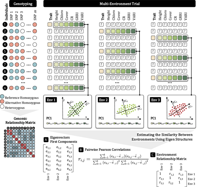
The environmental kernel $\varvec{E}$ was derived from image-based traits using a PCA-based approach to overcome the challenge of sparse testing, where not all genotypes are phenotyped in all environments. The procedure (summarized in Fig. 1) involved: (i) selecting only individuals with complete image-based data for each environment; (ii) performing PCA on the image-based traits within each environment; (iii) extracting the first principal component eigenvector as a summary of each environment; and (iv) computing pairwise Pearson correlations between environments based on these eigenvectors. The resulting correlation matrix was used as the kernel $\varvec{E}$.

Consider a set of m environments, where each environment i contains $n_i$ observations for six standardized image-based traits: VARI, GRRI, CR, coverage, height, and chlorophyll. For each environment i, let the random data matrix be denoted as $\varvec{X}_i\in \varvec{\mathbb {R}}^{n_i\times 6}$, with associated covariance matrix $\varvec{\Sigma }_i\in \varvec{\mathbb {R}}^{6\times 6}$.

Each covariance matrix $\varvec{\Sigma }_i$ has 6 eigenvalues ($\lambda _{1i}\ge \lambda _{2i}\ge \lambda _{3i}\ge \lambda _{4i}\ge \lambda _{5i}\ge \lambda _{6i}$) and corresponding normalized eigenvectors $e_{1i}$, $e_{2i}$, $e_{3i}$, $e_{4i}$, $e_{5i}$, $e_{6i}$. The first principal component score for environment i is then defined as:

$$\begin{aligned} \varvec{PC1}_i = e_{1i,1}\varvec{X}_{i,1}+e_{1i,2}\varvec{X}_{i,2}+e_{1i,3}\varvec{X}_{i,3}+e_{1i,4}\varvec{X}_{i,4}+e_{1i,5}\varvec{X}_{i,5}+e_{1i,6}\varvec{X}_{i,6} \end{aligned}$$

(9)

where $e_{1i,j}$ denotes the j-th component of the first eigenvector $e_{1i}$, and $\varvec{X}_{i,j}$ is the vector of observations for trait j in environment i.

The first eigenvectors for all environments are assembled into a matrix:

$$\begin{aligned} \varvec{E}_1=\left[ \varvec{e}_{1,1}, \varvec{e}_{1,2}, …, \varvec{e}_{1,m}\right] , \end{aligned}$$

(10)

where each column $\varvec{e}_{1,i}$ represents the first eigenvector from environment i. Pairwise Pearson correlations are then computed between the columns of $\varvec{E}_1$, and the resulting correlation coefficients define the entries of the environmental kernel $\varvec{E}$.

Source link

Phenomics-assisted sparse testing for potato breeding